Post Outline

Recap
Hypothesis
Strategy
Conclusion
Caveats and Areas of Exploration
References

Recap

In Part 1 we learned about Hidden Markov Models and their application using a toy example involving a lazy pet dog. In Part 2 we learned about the expectation-maximization algorithm, K-Means, and how Mixture Models improve on K-Means weaknesses. If you still have some questions or fuzzy understanding about these topics, I would recommend reviewing the prior posts. In those posts I also provide links to resources that really helped my understanding.

Hypothesis

Given what we know about Mixture Models and their ability to characterize general distributions, can we use it to model a return series, such that we can identify outlier returns that are likely to mean revert?

Strategy

This strategy attempts to predict an asset's return distribution. Actual returns that fall outside the predicted confidence intervals are considered outliers and likely to revert to the mean.

We first fit a Gaussian Mixture Model to the historical daily return series. We use the model's estimate of the hidden state's mean and variance as parameters to a random sampling from the JohnsonSU distribution. We then calculate confidence intervals from the sampled distribution.

From there we evaluate model accuracy and the n days cumulative returns after each outlier event. We compute some summary statistics and try to answer the hypothesis.

Why the johnson SU distribution?

Searching the net I found a useful bit of code from this site. Instead of assuming our asset return distribution is normal, we can use Python and Scipy.stats to find the brute force answer. We can cycle through each continuous distribution and run a goodness-of-fit procedure called the KS-test. The KS-test is a non-parametric method which examines the distance between a known cumulative distribution function and the CDF of the your sample data. The KS-test outputs the probability that your sample data comes from the benchmark distribution.

After running this code you should see output similar to the below code. For simplicity sake, just remember the higher the p-value, the more confident the ks-test is that our data came from the given distribution.

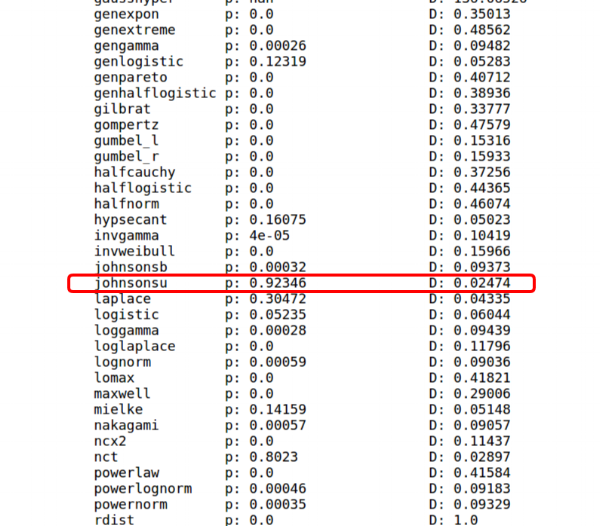
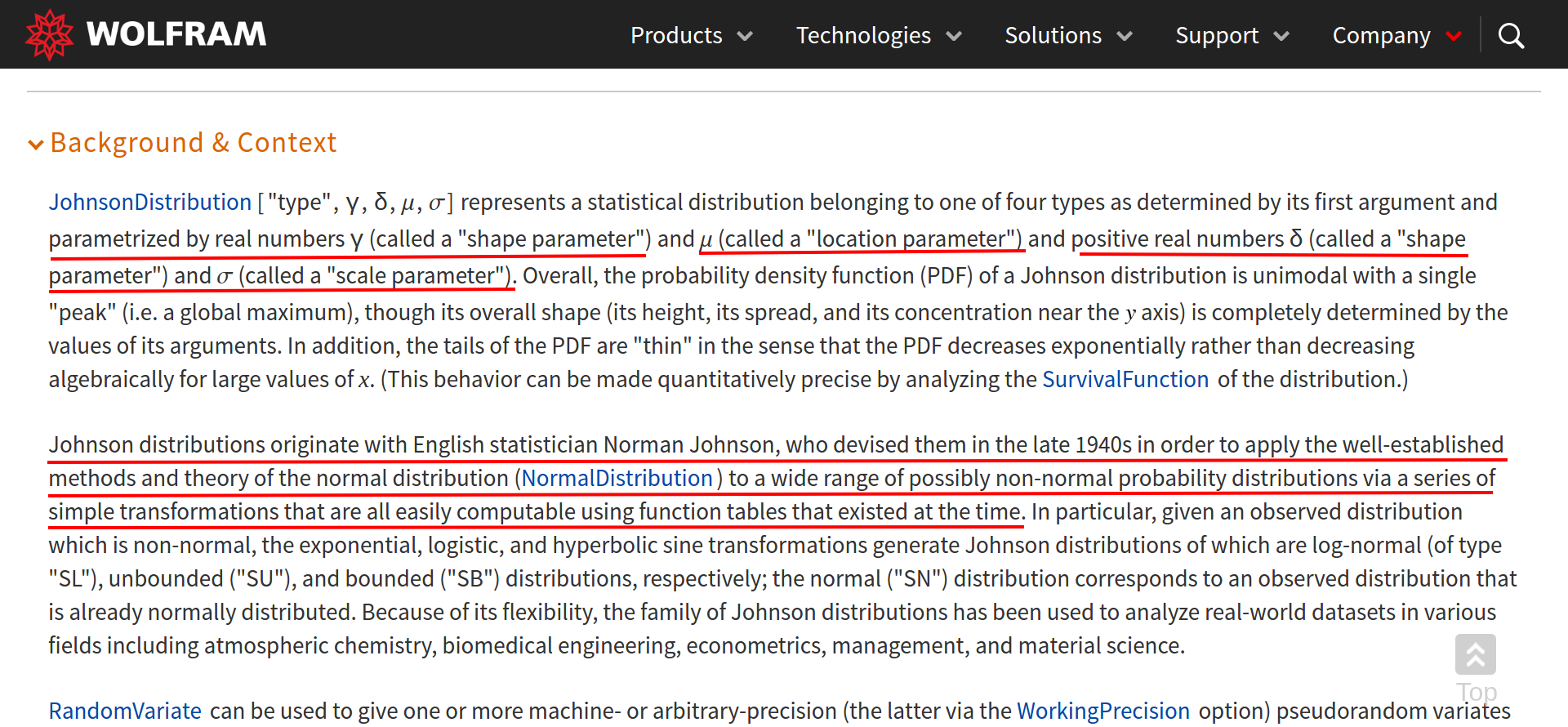
I had never heard of the Johnson SU distribution before this code. I had to research it, and I found that the Johnson SU was developed to in order to apply the established methods and theory of the normal distribution to non-normal data sets. What gives it this flexibility is the two shape parameters, gamma and delta, or a, b in Scipy. For more information I recommend this Wolfram reference link and this Scipy.stats link.

After selecting the distribution we can code up the experiment.

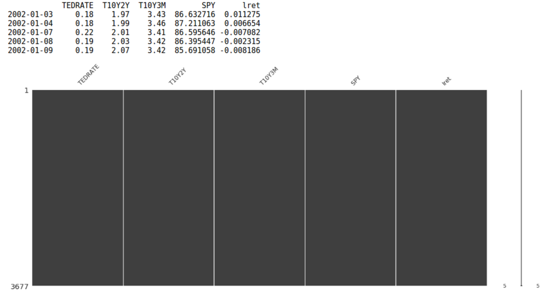
Now let's get some data.

Now we create our convenience functions. The first is the run_model() function which takes the data, feature columns, and Sklearn mixture parameters to produce a fitted model object and the predicted hidden states. Note that you can use a Bayesian Gaussian mixture if you so choose. The difference between the two models is that the Bayesian mixture model will try to derive the correct number of mixture components up to a chosen maximum. For more information on the Bayesian mixture model I recommend consulting the Sklearn docs.

The next function takes the model object and predicted hidden states and returns the estimated mean and variance of the last state.

Now we take the estimated state mean and variance of the last predicted state and feed it into the _get_ci() function. This function takes the alpha and shape parameters, estimated mean and variance and randomly samples from the JohnsonSU distribution. From this distribution we derive confidence intervals.

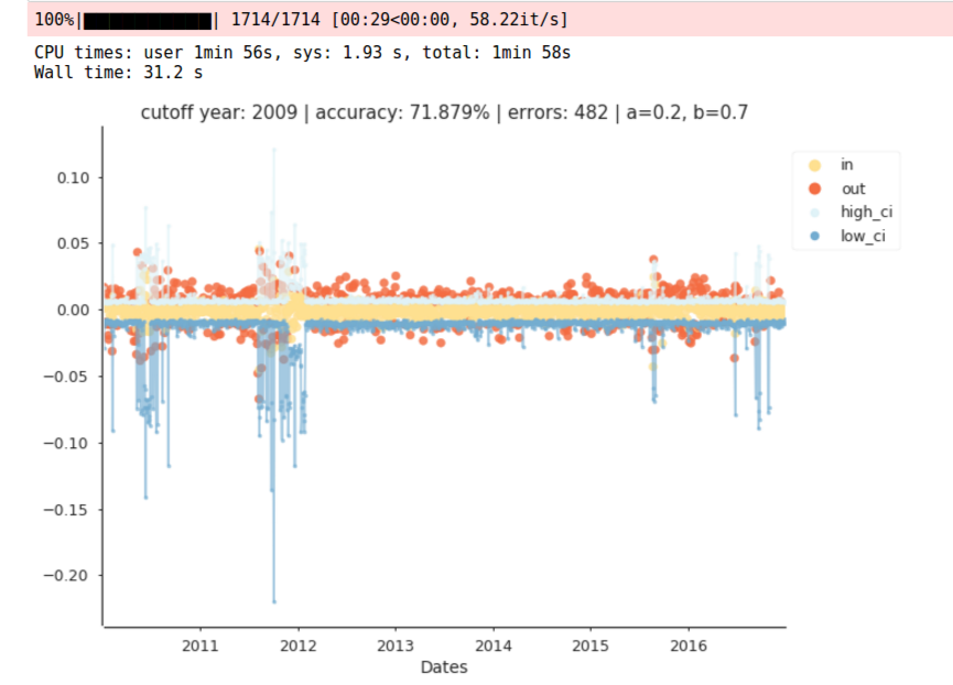
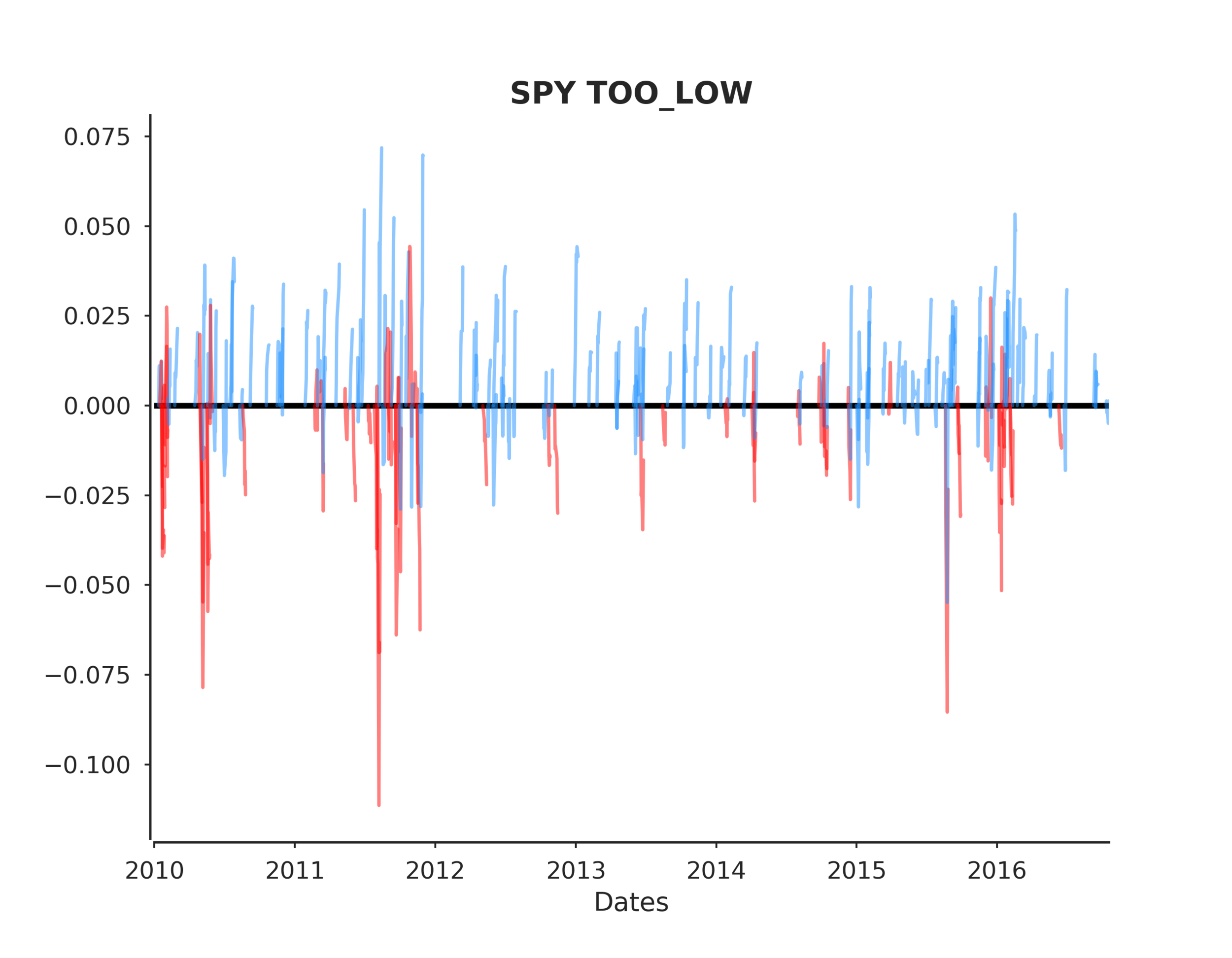
The final function visualizes our model predictions, by highlighting target returns that fell inside and outside the confidence intervals, along with our predicted confidence intervals.

Now we can run the model in a walk-forward fashion. The code uses a chosen lookback period up until the cutoff year to fit the model. From there, the code iterates refitting the model each day, outputting the predicted confidence intervals. The code is setup to run using successive cutoff years, however I will leave that to you readers to experiment with. In this demo we will break the loop after the first cutoff year.

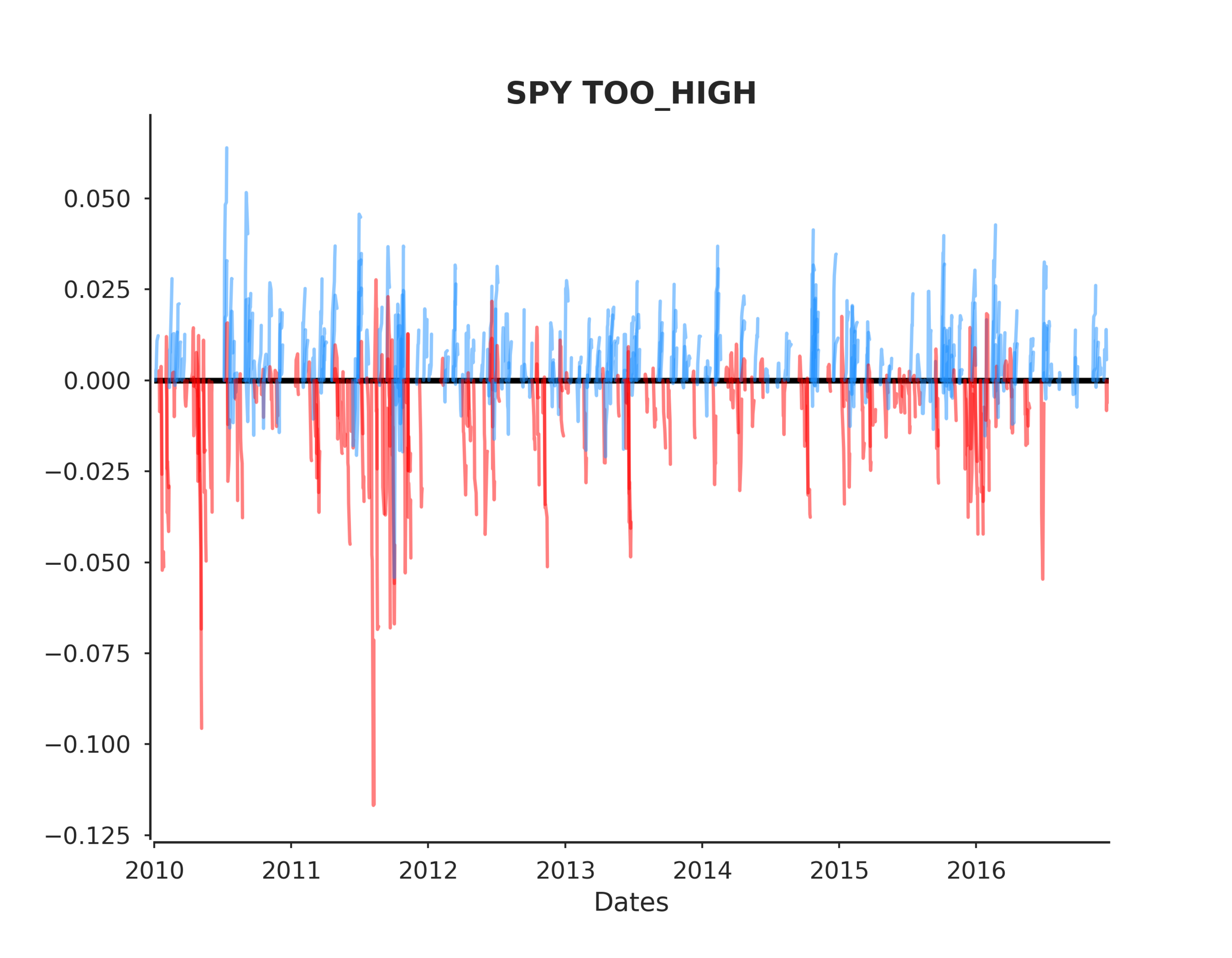
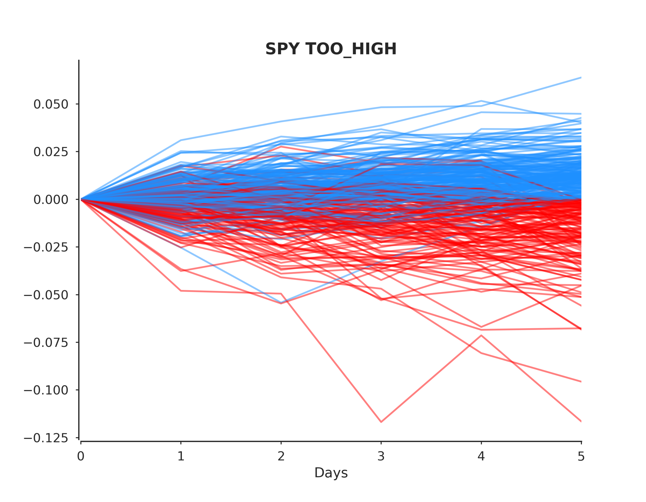
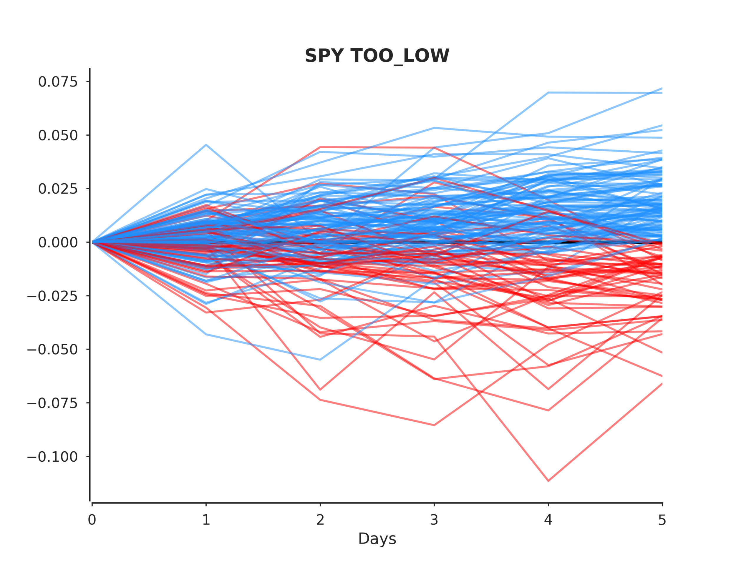
After that's complete we need to set up our analytics functions to evaluate the return patterns post each event. Recall that an event is an actual return that fell outside of our predicted confidence intervals.

Now we can run the following code to extract the events, output the plots and view the summary.

Conclusions

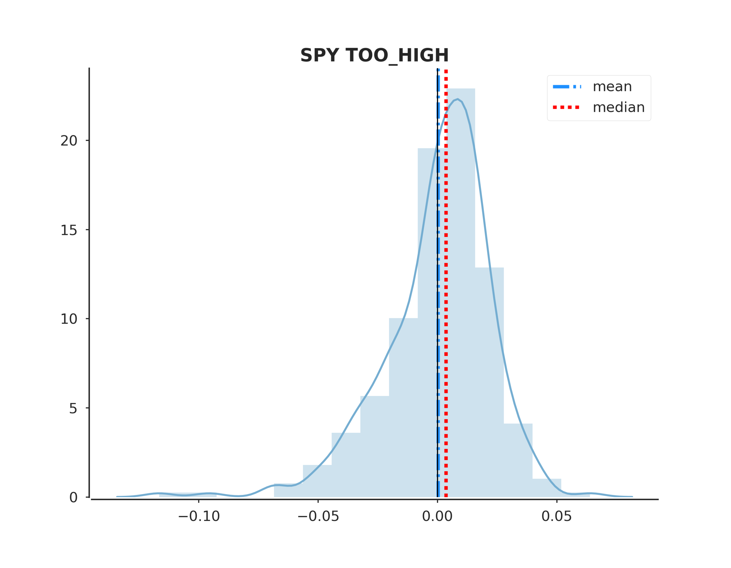
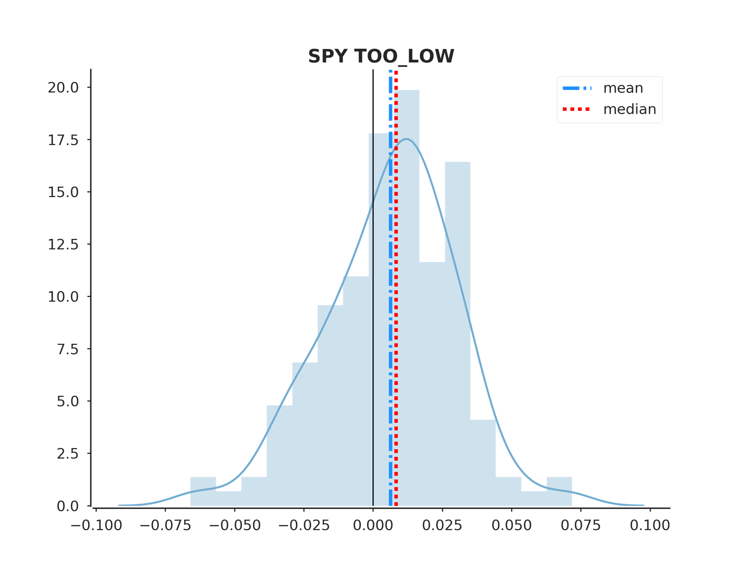
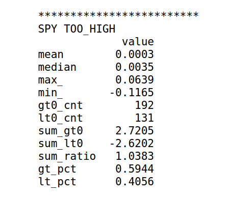
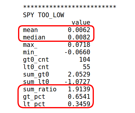
To answer the original hypothesis about finding market bottoms, we can examine the returns after a too low event. Looking at the summary we can see that the mean and median return are +62 and +82 bps respectively. Looking at the sum_ratio we can see that that the sum of all positive return events is almost 2x the sum of all negative returns. We can also see that, given a too low event, after 5 days SPY had positive returns 65% of the time!

These are positive indicators that we may be able to predict market bottoms. However, I would emphasize more testing is needed.

Caveats and Areas of Exploration

We don't consider market frictions such as commissions or slippage
The daily prices may or may not represent actual traded values.
I used a coarse search to find the JohnsonSU shape parameters, a and b. These may or may not be the best values. Just note that we can use these parameters to arbitrarily adjust the confidence intervals to be more or less conservative. I leave this for the reader to explore.
In many cases both too high, and too low events result in majority positive returns, this could be an indication of the overall bullishness of the sample period that may or may not affect model results in the future.
I chose k=2 components for computational simplicity, but there may be better values.
I chose the lookback period for computational simplicity, but there may be better values.
Varying the step_fwd parameter may hurt or hinder the strategy.
What makes this approach particularly interesting, is that we don't want anything close to 100% accuracy from our predicted confidence intervals, otherwise we won't have enough "trades". This adds a level of artistry/complexity because the parameter values we choose should create predictable mean reversion opportunities, but the model accuracy is not a good indicator of this. Testing the strategy with other assets shows "profitability" in some cases where the model accuracy is sub 60%.

Please contact me if you find any errors.

Can We Use Mixture Models to Predict Market Bottoms?