Post Outline

• Recap
• Model Update
• Model Testing
• Model Results
• Conclusions
• Code

Recap

In the previous post I gave a basic "proof" of concept, where we designed a trading strategy using Sklearn's implementation of Gaussian mixture models. The strategy attempts to predict an asset's return distribution such that returns that fall outside the predicted distribution are considered outliers and likely to mean revert. It showed some promise but had many areas in need of improvement.

Model Update

In this version I've refactored a lot of the code into a more object oriented structure. Now the code uses three classes.

1. ModelRunner() class - This is the class for executing the model and returning our prediction dataframe and some key parameters.
2. ResultEval() class - This takes the data from the prediction dataframe and key parameters and outputs our strategy returns and summary information.
3. ModelPlots() class - This takes our data and outputs key plots to help visualize the strategy performance.

I did this for several reasons.

• Reduce the likelihood of input errors by creating objects that share parameters.
• Increase the ease of model testing.
• Increase interpretability.

Model Testing

In this version, we are going to expand the analysis to include other, actively traded ETFs, and test the reproducibility of the results, and generalization ability of the model.

Here are the ETFs we will examine: symbols = ['SPY', 'DIA', 'QQQ', 'GLD', 'TLT', 'EEM', 'ACWI']

Assuming the correct imports, with the refactored code we can run the model in the following fashion. We'll focus on the TOO_LOW events although I encourage readers to experiment with both.

In this post I'm going to skip to the results and conclusions, and provide the refactored code at the end.

Model Results

First let's look at the model results using SPY.

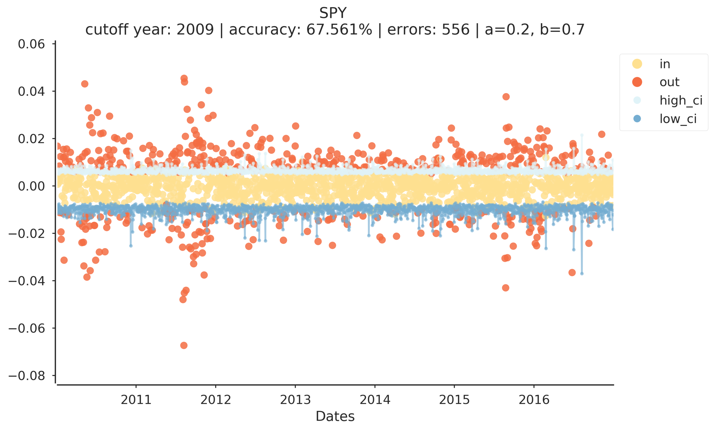
The first thing I noticed was that the confidence intervals were less responsive to increases in return volatility. The difference shows up in the reduction in accuracy. In Part 1, I believe the accuracy was ~71% whereas in the updated model the accuracy has dipped to ~68%! Does that hurt our strategy?

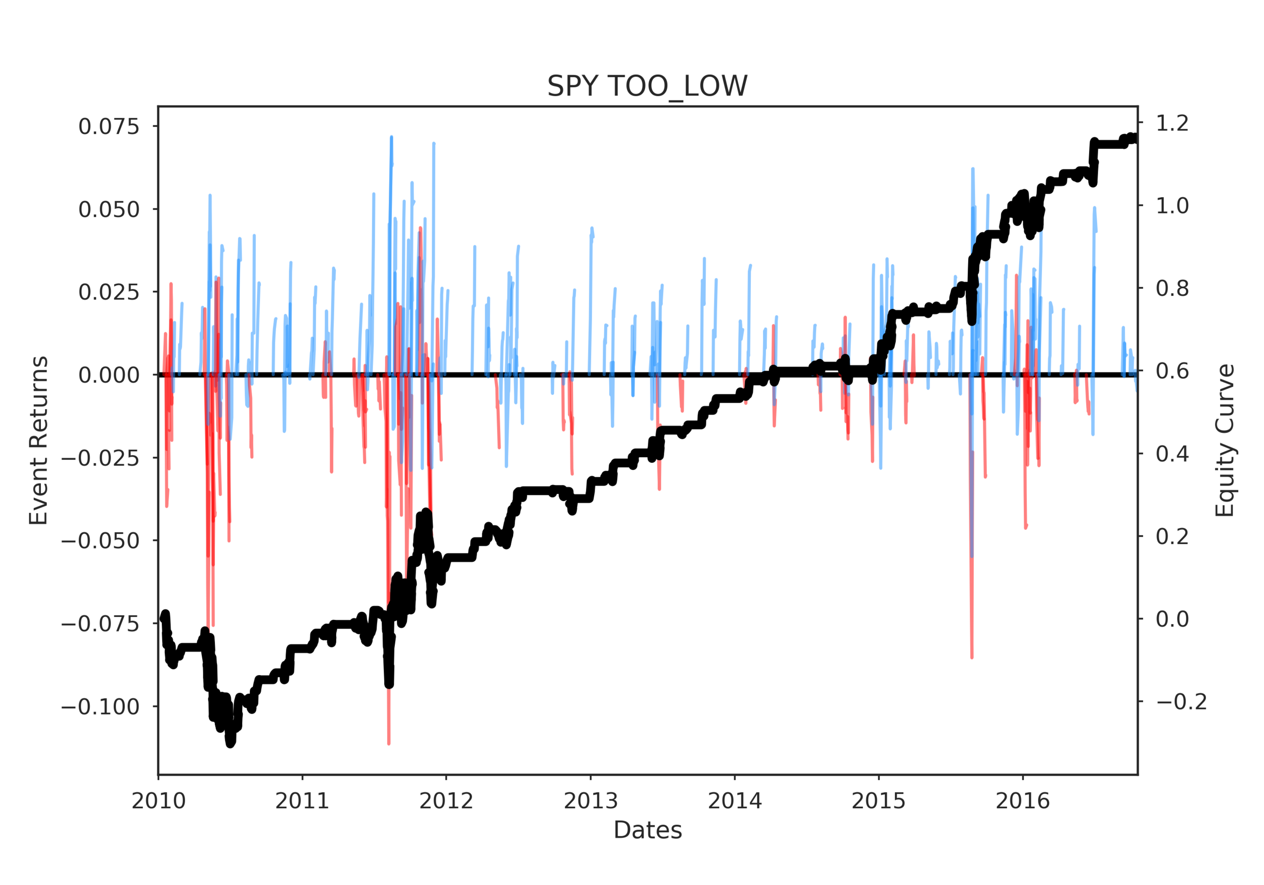
Judging by the equity curve, our strategy is not noticeably impacted by the reduced model accuracy!

The plotted equity curve is the cumulative sum of each event's returns assuming every event was a "trade". This should include overlapping events.

Let's look at the model results for the other ETFs.

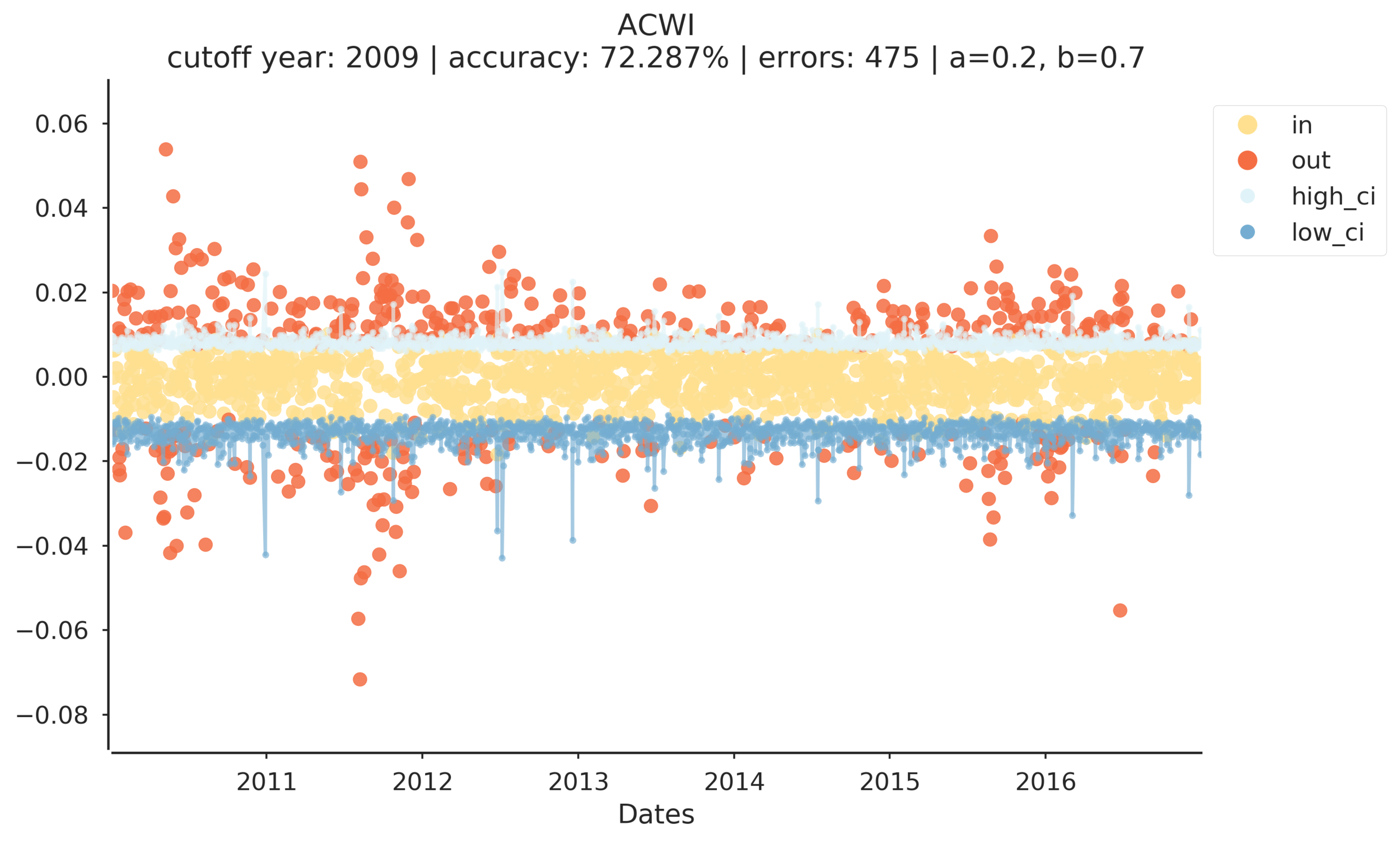
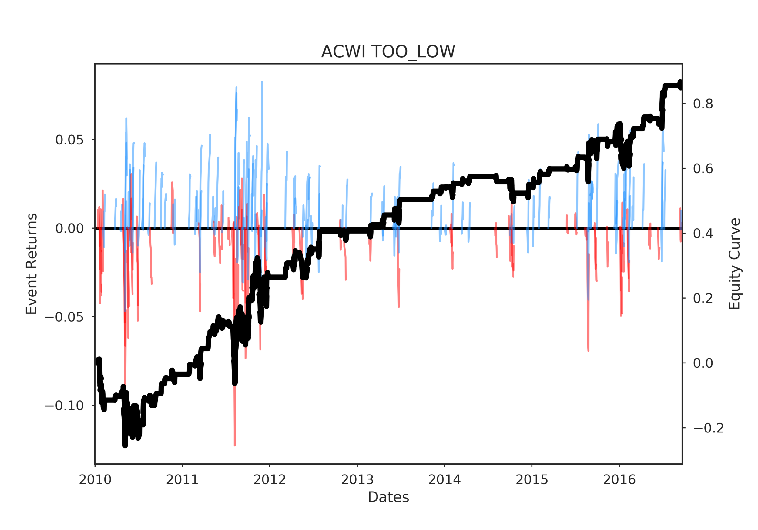
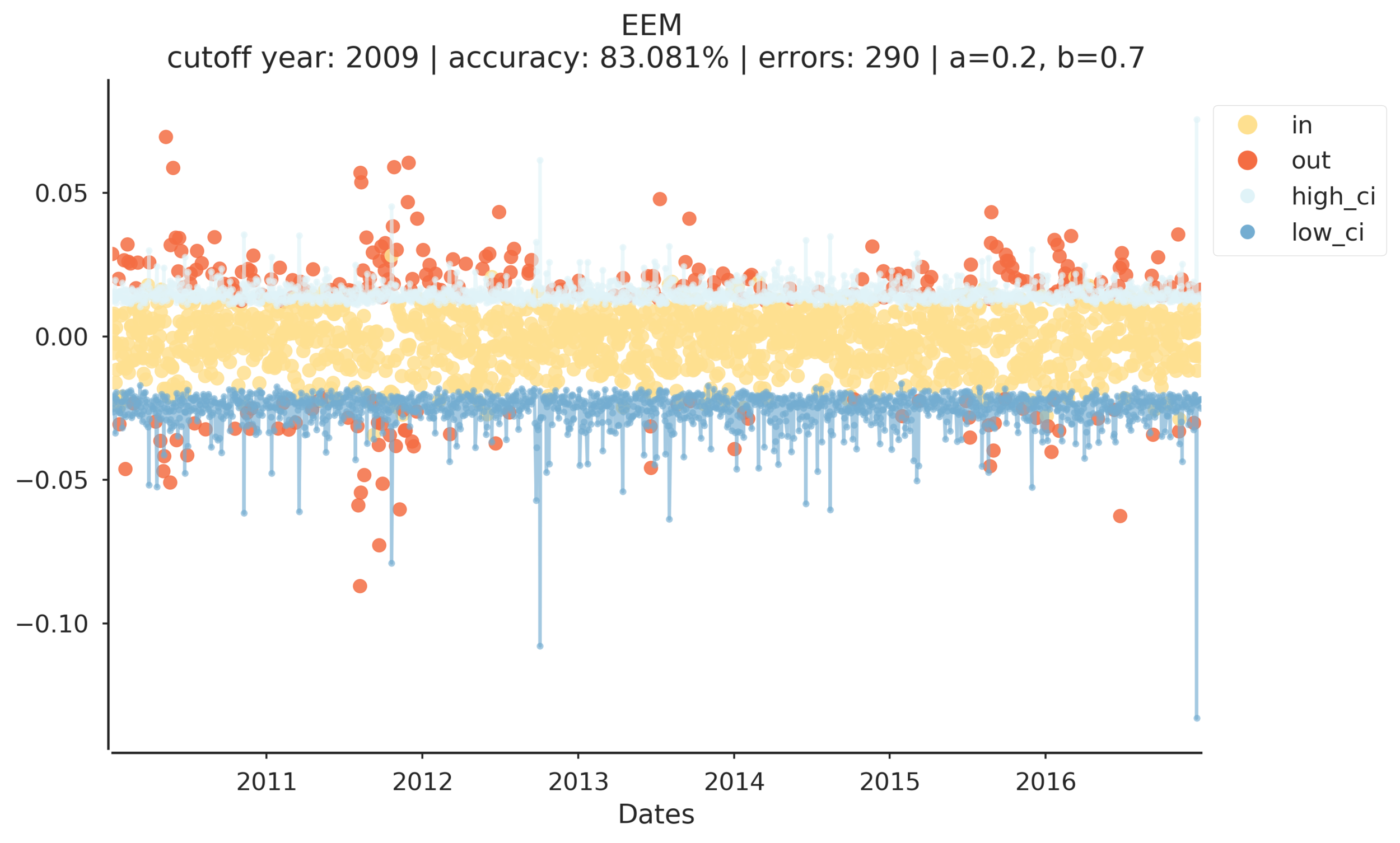
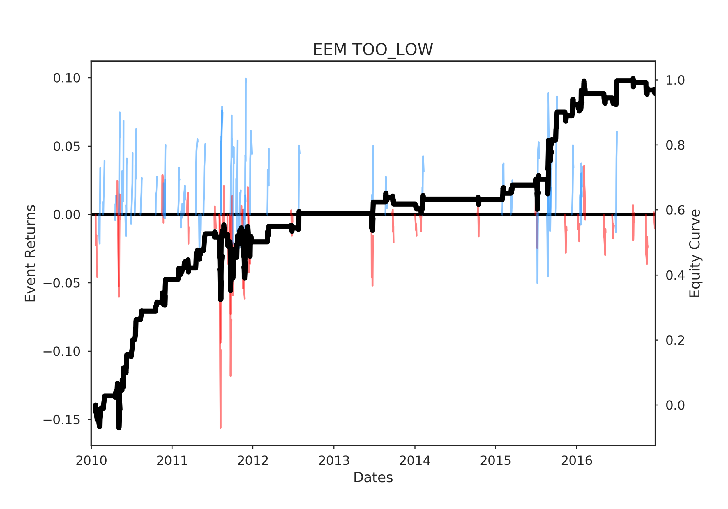
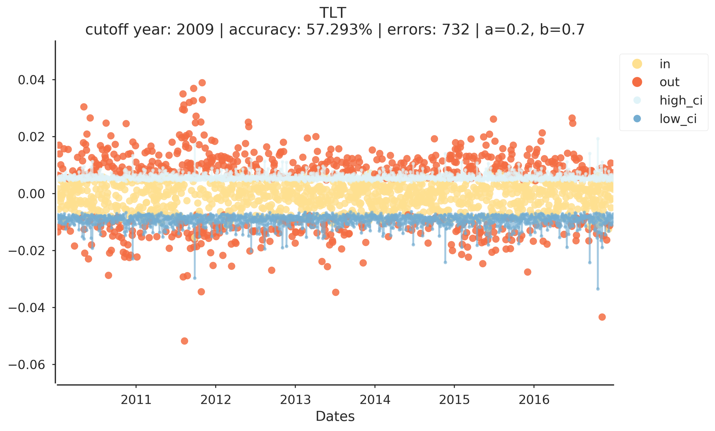
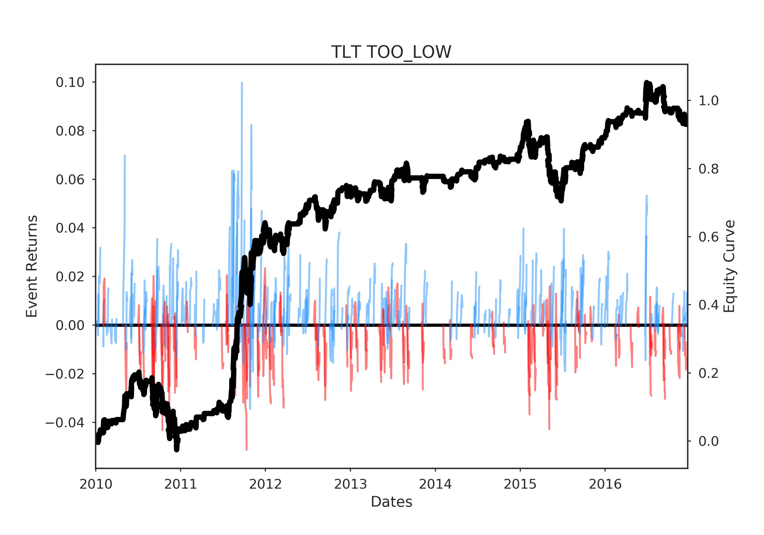
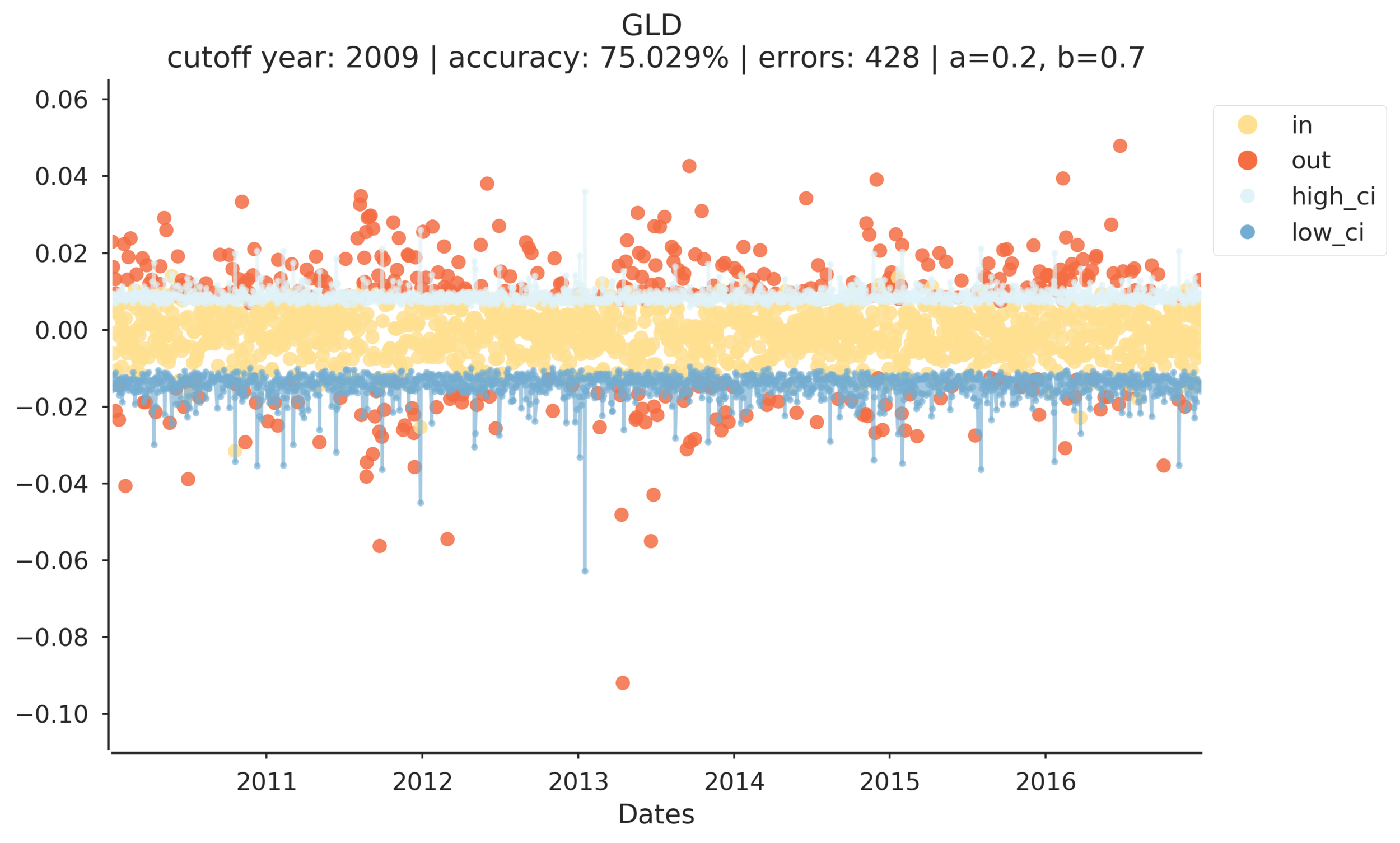
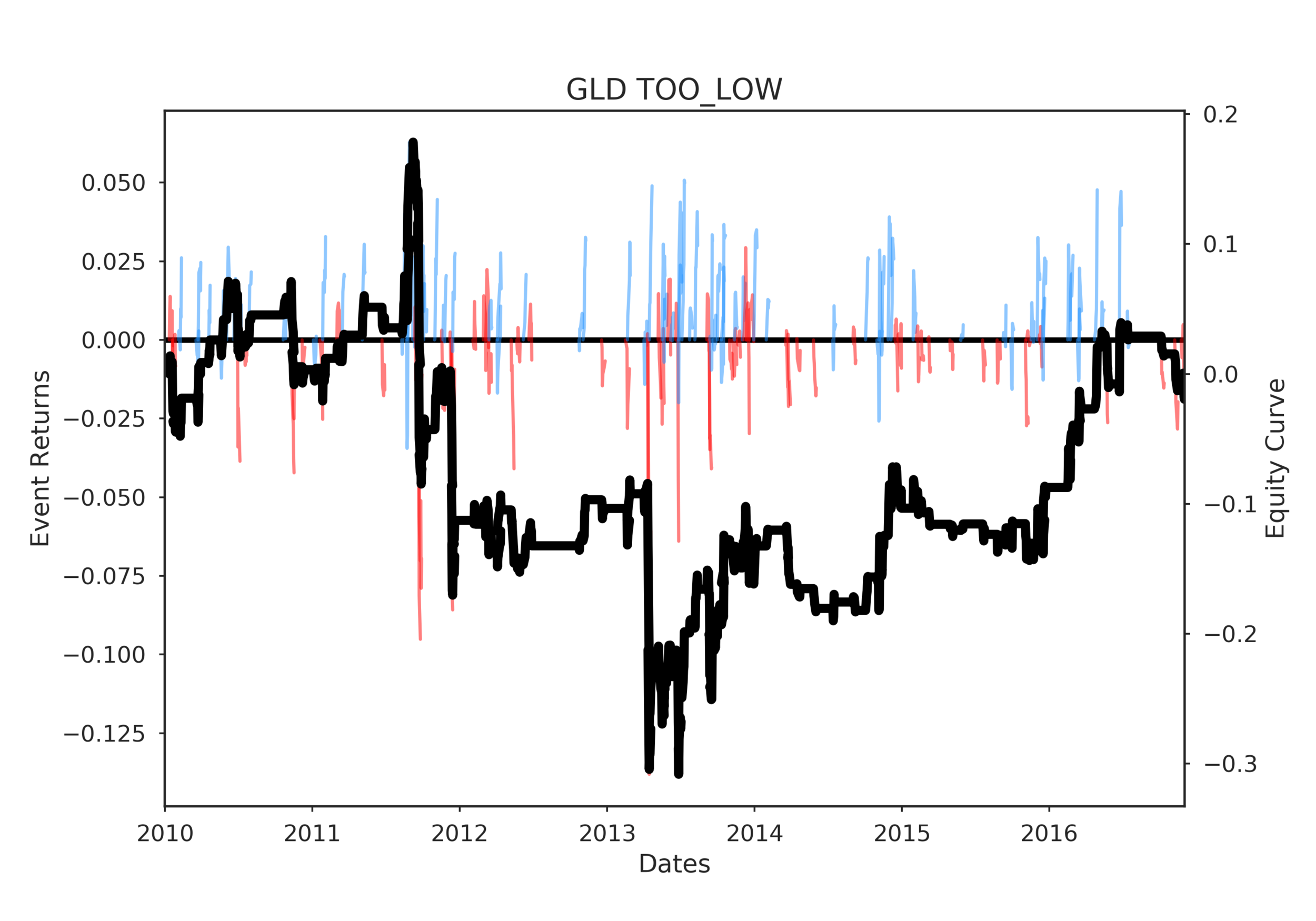
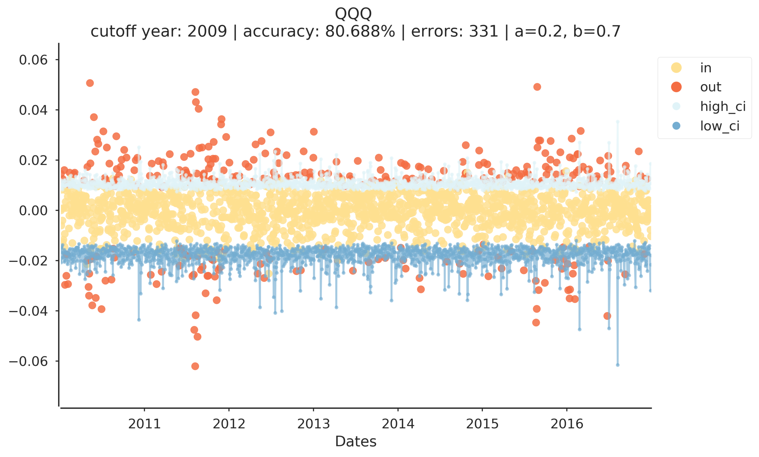
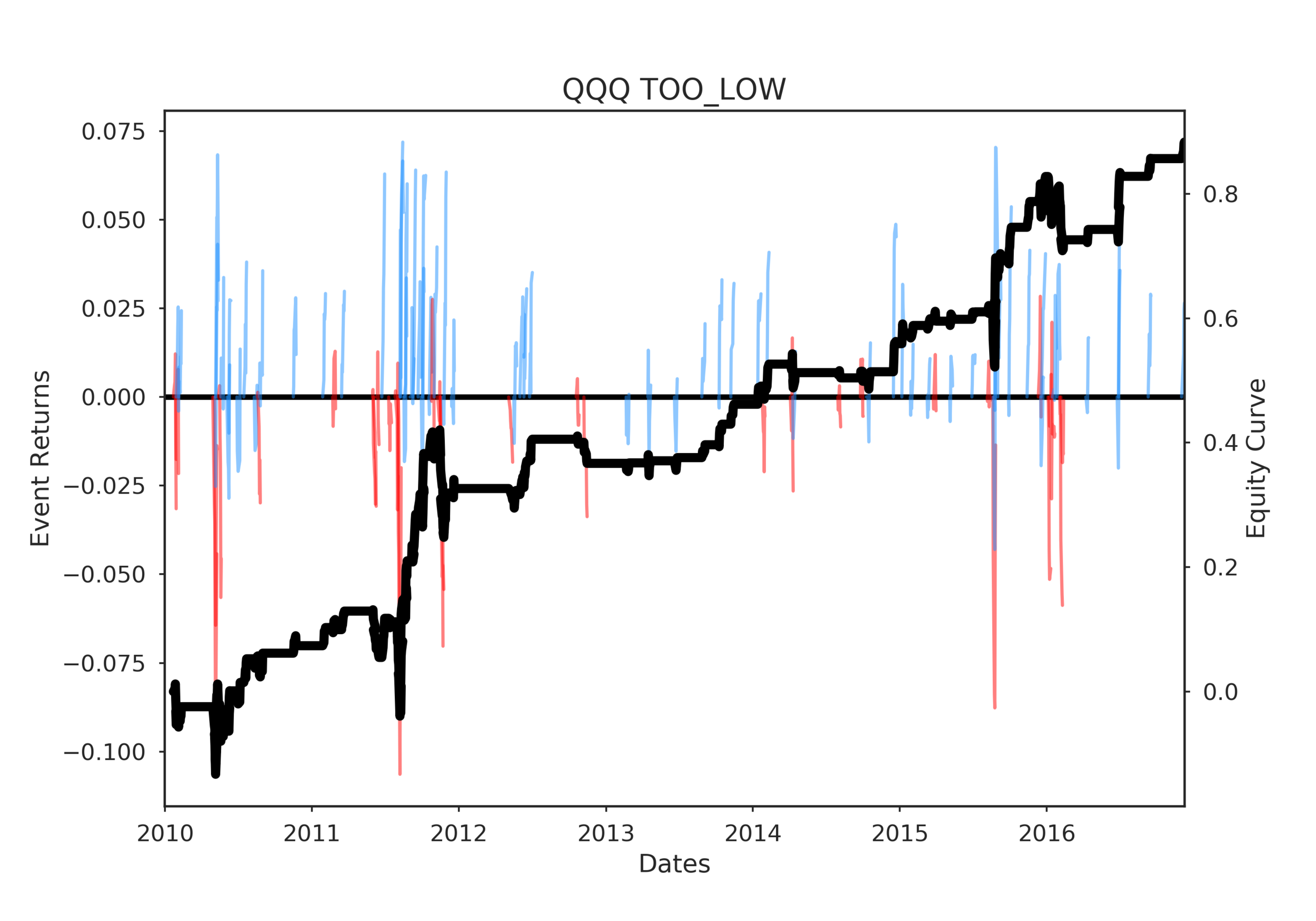
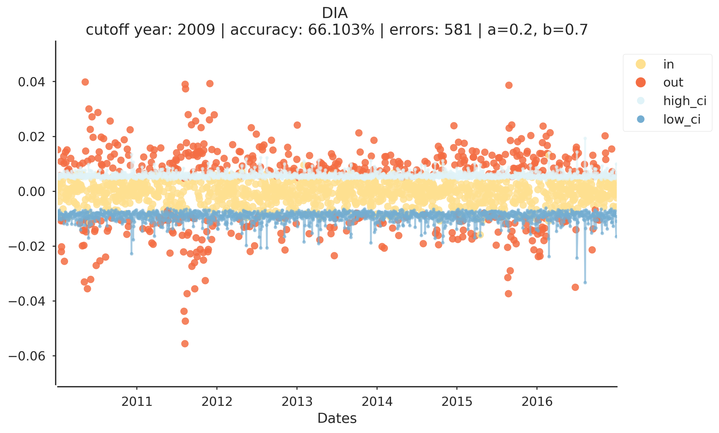
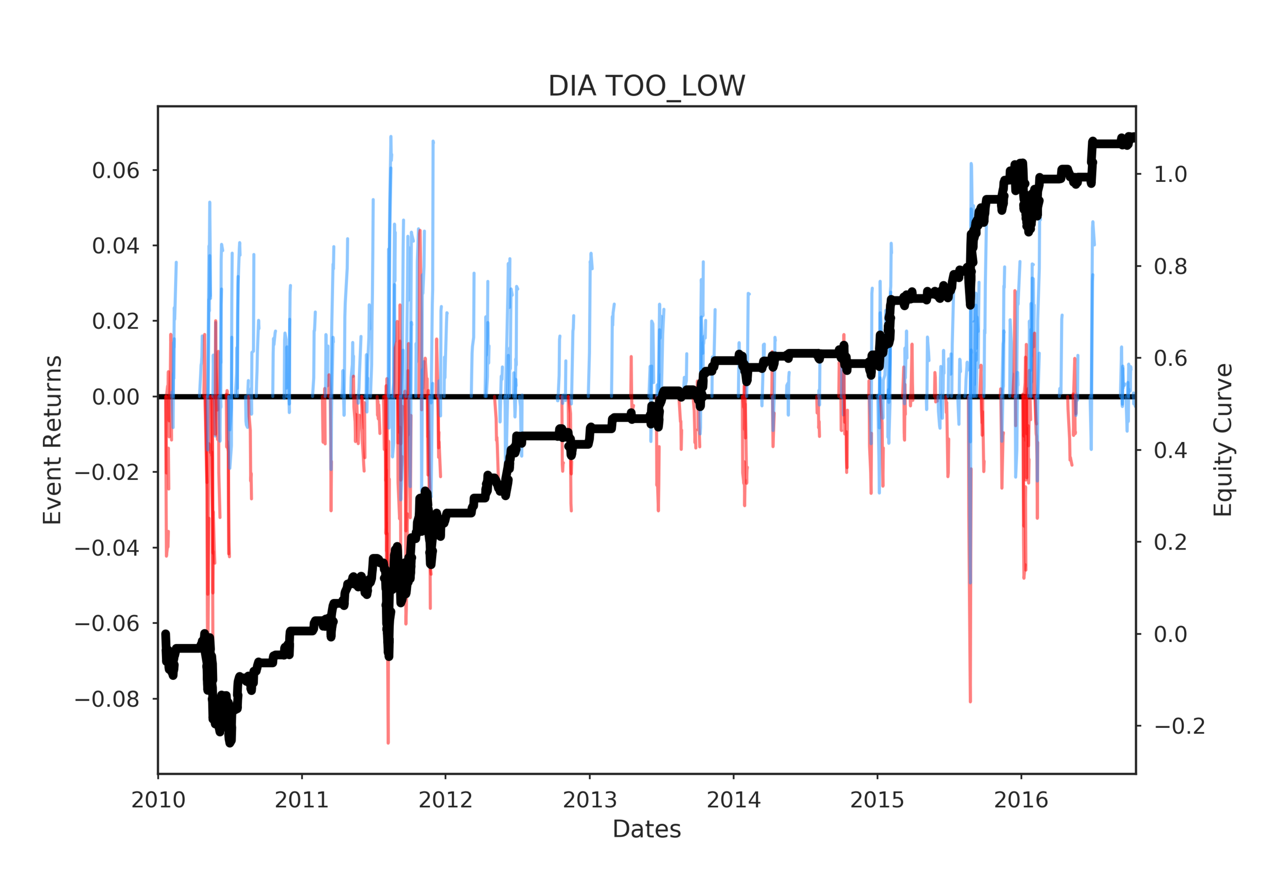
The model has some interesting output. Notice that model accuracy ranges from ~57% (TLT) to ~83% (EEM). However, both of these equity curves end positively. GLD is distinctly volatile, and ends poorly, however the model was 75% accurate. DIA, QQQ, SPY, and ACWI all have stable sharply positive equity curves.

Conclusions

This supports my initial findings that model accuracy seems loosely, if at all, related to the strategy's equity curve. These results do indicate that the strategy is worth further evaluation but I'm hesitant to declare success.

I need to test the strategy over a longer period of time and make sure to include 2008/9. Also, I need to drill down into evaluating the strategy results vs the correlation of asset returns. For example, DIA, QQQ, and SPY are highly correlated, so we would expect the strategy to have similar results among those ETFs, but what about negatively and uncorrelated assets? TLT is generally negatively correlated with SPY while GLD is likely uncorrelated. Is the strategy performance for those two ETFs representative of other negatively/uncorrelated ETFs?

Code