How to get Free Intraday Stock Data with Python and BarCharts OnDemand API

To this day the most popular article I have ever written on this blog was "How to get Free Intraday Stock Data with Netfonds". Unfortunately the Netfonds API has really declined in terms of usability, with too many popular stocks missing, and irregular trade and price quotes. Simply put, as the API went down, so did the code.

However, all hope is not lost. The wonderful people at BarChart.com have created a well documented, easily accessible API for intraday stock data and even near real-time quote access. The only caveat is that you must request access to get a personal API key. Again this is FREE, and the process is extremely simple and straightforward. I think I received my API key within the same day, max 24 hours. 

Step 1: Go to http://www.barchartondemand.com/api.php and request an API key. 

Step 2: Use or modify my code to get FREE intraday stock data. 

Something to note, in this example I use the SP500 components as my list of stock symbols. I covered how to get fresh SPY holdings data directly from the provider in a previous post titled "GET FREE FINANCIAL DATA W/ PYTHON (STATE STREET ETF HOLDINGS - SPY)".  Now onto the code...

First I import the necessary modules.


# -*- coding: utf-8 -*-
import time
t0 = time.clock()

import pandas as pd
from pandas.tseries.offsets import BDay
import numpy as np
import datetime as dt
from copy import copy
import warnings
warnings.filterwarnings('ignore',category=pd.io.pytables.PerformanceWarning)

Next I set up what I refer to as a 'datetime management' section of my code. I do this for ALL my time series analysis as a convenient way to standardize my code across projects. Sometimes I only use one of the variables, as I do in this case, but it's so convenient when doing any sort of exploratory analysis with time series. I also do the same for my filepaths.


# ================================================================== #
# datetime management

d = dt.date.today()
# ---------- Days ---------- 
l10 = d - 10 * BDay()
l21 = d - 21 * BDay()
l63 = d - 63 * BDay()
l252 = d - 252 * BDay()
# ---------- Years ---------- 
l252_x2 = d - 252 * 2 * BDay() 
l252_x3 = d - 252 * 3 * BDay() 
l252_x5 = d - 252 * 5 * BDay()
l252_x7 = d - 252 * 7 * BDay() 
l252_x10 = d - 252 * 10 * BDay() 
l252_x20 = d - 252 * 20 * BDay() 
l252_x25 = d - 252 * 25 * BDay()

# ================================================================== #
# filepath management

project_dir = r'D:\\' 
price_path = project_dir + r'Stock_Price_Data\\'

Next I set up a convenience function for creating the BarChart url to access the API. 


# ================================================================== #
apikey = 'insert_your_api_key'
def construct_barChart_url(sym, start_date, freq, api_key=apikey):
    '''Function to construct barchart api url'''
    
    url = 'http://marketdata.websol.barchart.com/getHistory.csv?' +\
            'key={}&symbol={}&type={}&startDate={}'.format(api_key, sym, freq, start_date)
    return url

Now for the fun part. I create a function that does the following:

  1. initializes an empty dictionary and the minimum required API variables,
  2. iterates through my list of SP500 stocks,
  3. constructs the proper API url,
  4. reads the data returned by the db as a csv file conveniently making use of Pandas read_csv function.
  5. adds the price dataframe to the dictionary dynamically
  6. converts the python dictionary into a Pandas Panel and returns the Panel

def get_minute_data():
    '''Function to Retrieve <= 3 months of minute data for SP500 components'''
    
    # This is the required format for datetimes to access the API
    # You could make a function to translate datetime to this format
    start = '20150831000000'
    #end = d
    freq = 'minutes'    
    prices = {}
    symbol_count = len(syms)
    N = copy(symbol_count)
    try:
        for i, sym in enumerate(syms, start=1):
            api_url = construct_barChart_url(sym, start, freq, api_key=apikey)
            try:
                csvfile = pd.read_csv(api_url, parse_dates=['timestamp'])
                csvfile.set_index('timestamp', inplace=True)
                prices[sym] = csvfile
            except:
                continue
            N -= 1
            pct_total_left = (N/symbol_count)
            print('{}..[done] | {} of {} symbols collected | percent remaining: {:>.2%}'.format(\
                                                                sym, i, symbol_count, pct_total_left)) 
    except Exception as e: 
        print(e)
    finally:
        pass
    px = pd.Panel.from_dict(prices)

    return px

Now I import our list of stock symbols, make some minor formatting edits and run the code.


# ================================================================== #

# header=3 to skip unnecesary file metadata included by State Street    
spy_components = pd.read_excel(project_dir +\
                             '_SPDR_holdings/holdings-spy.xls', header=3)
syms = spy_components.Identifier.dropna()
syms = syms.drop(syms.index[-1]).order()

pxx = get_minute_data()

This script takes roughly 40 minutes to run, longer if you try to get the full 3 months they provide, less if you need less data. 

Now let's test our output to make sure we got what we expected. 


print(pxx)
print(pxx['AAL'].tail())
print(pxx['ZTS'].tail())

The code ran correctly it appears, and the output is what we expected. One thing you may have noticed is that time stamps are not 'EST'. If you want to convert them use the following one liner. 


# convert timestamps to EST
pxx.major_axis = pxx.major_axis.tz_localize('utc').tz_convert('US/Eastern')

There is one last consideration that is easy to overlook if you're unfamiliar with some of the technical challenges of 'big data'. When you first run a script like this it is tempting to use the usual storage techniques that pandas provides such as 'pd.to_csv()' or 'pd.to_excel()'. However, consider the volume of data we just collected: 502 (items) x 5866 (major_axis) x 7 (minor_axis) = 20,613,124. 

Look at it again and consider this simple code collected over 20 million data points! I ran into trouble with Python/Excel I/O with only 3.5 million data points in the past. Meaning importing and exporting the data took minutes. That's a serious hangup for any type of exploratory research, especially if you plan on sharing and/or collaborating using this dataset. 

Pandas HDF5 file storage format to the rescue! Feel free to investigate the power, speed and scalability of HDF5 via the Pandas docs or any of the numerous quality blogs out there accessible by a google search. Needless to say, I/O was reduced from several minutes both ways to seconds. Here is the code I used to store the panel.  


try:
    store = pd.HDFStore(price_path + 'Minute_Symbol_Data.h5')
    store['minute_prices'] = pxx
    store.close()
except Exception as e:
    print(e)
finally:
    pass

Here's a sample plot with the intraday data. 

The entire code is posted below using Gist.

Guest Post Previously Featured on RectitudeMarket.com (09/02/2015)

**Note: This post already appeared as a guest post on rectitudemarket.com. The reason I'm posting this article when it is 'outdated', is twofold. 1) I think it's beneficial to review previous works especially when one has the benefit of hindsight. This helps us determine the accuracy and bias of the research presented. 2) I further introduce the concept of conditional cumulative returns, which adds insight to what happens to our securities' returns given some other event occurring. In this case, the event is simply whether our benchmark ETF's cumulative returns are rising or falling during some period. 

Are There Any Equity Industry Groups Outperforming During this Recent Market Volatility?

Stock market volatility has picked up in a big way. It has been some time since market participants have experienced consecutive 2-4% up/down moves in the major market averages. The selling has been broad based and market sentiment has deteriorated as well.

With this backdrop I wondered if any industry groups were doing well. By doing well I mean 1) relative outperformance when compared to other industries 2) absolute performance greater than zero.

To answer this question I collected all the NYSE and Nasdaq symbols (~3300 symbols), filtered them for firms with a market cap greater than $300 million then I grouped them by industry. I dropped any industries with less than 10 stock symbols. With the filtered dataset I ran the analysis.

First I examined the cumulative return momentum over various lookback periods. Then I examined which industry groups had the best cumulative return performance given a benchmark ETF’s returns are rising (declining).

The benchmark ETF’s I selected for comparison are (SPY, QQQ, VTI). 

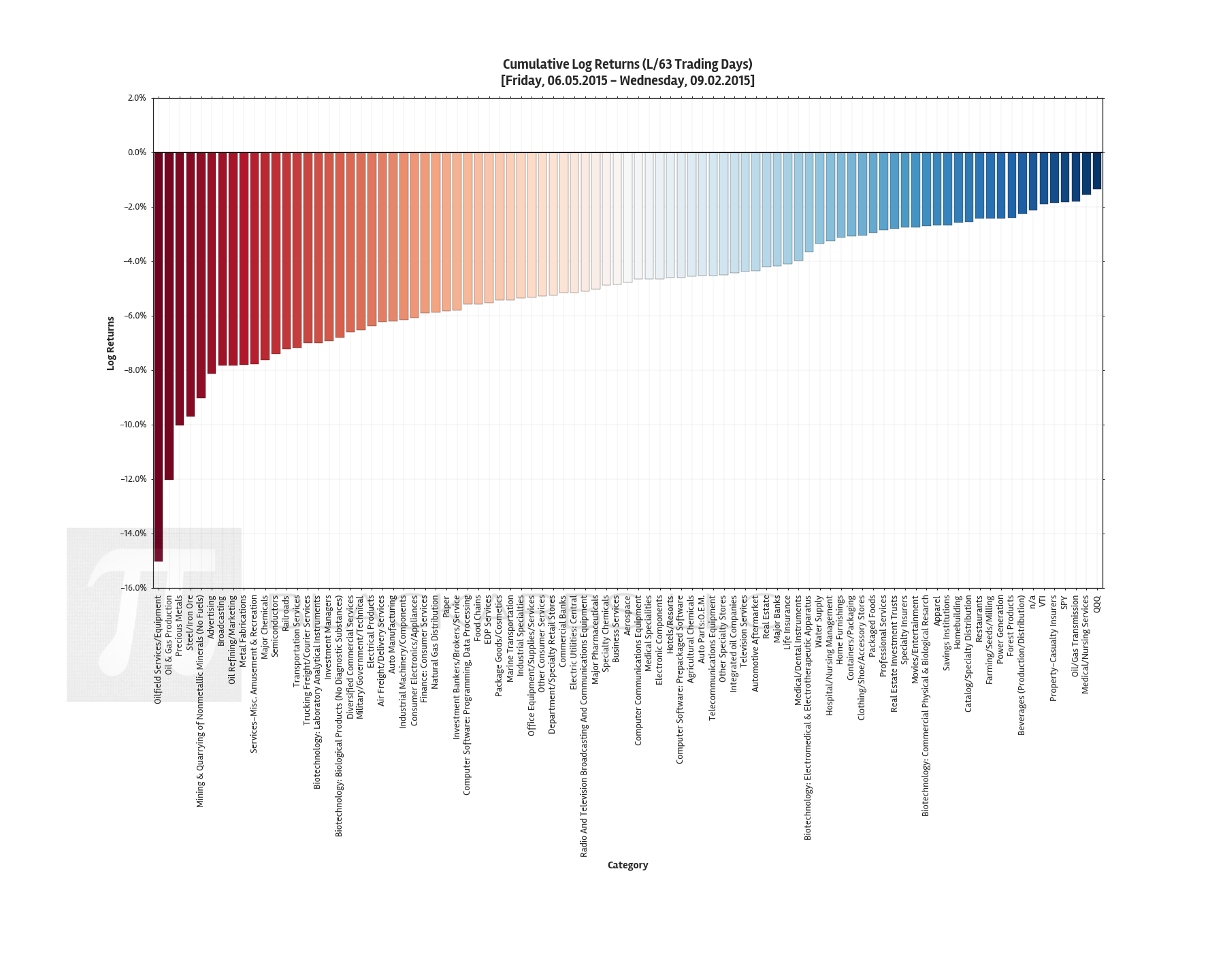
Unfortunately there are no industry groups with absolute cumulative return performance greater than zero over the last quarterly period (Last 63 Trading Days).

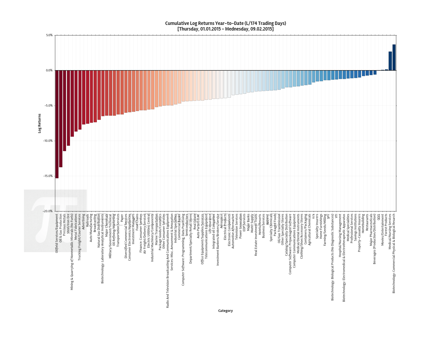
In fact you'd have to back out to view industry group performance Year-to-Date, to find any industry groups with positive cumulative returns. Those industries are: Biotechnology: Commercial Physical & Biological Research, Medical/Nursing Services, Forest Products,  and Movies/Entertainment.

To examine relative conditional performance, I selected the top 5% of industry group cumulative return performance given increasing benchmark returns (Last 63 Trading Days)

Focusing on SPY, the strongest performers given increasing returns have been: Finance: Consumer Services, Investment Bankers/Brokers/Service, Investment Managers, and Clothing/Shoe/Accessory Stores. Clearly financial firms’ returns are highly sensitive to the performance of SPY.  Somewhat surprisingly Clothing/Shoe/Accessory Stores have outperformed given increasing returns in all 3 benchmark ETFs.

For long only investors, unfortunately there are no industries which have recorded positive absolute cumulative return performance given a decline in benchmark returns. The best one can hope for is to find industries that decline less than peers during periods of negative market returns. 

During the last quarter (Last 63 Trading Days) the best industry performance given declining returns in SPY are: Life Insurance, Auto Parts 0.E.M., Computer Software: Prepackaged Software, and Business Services. I find it surprising that Business Services would be a relative outperformer for all 3 benchmark ETFs.

Another item of note is precious metals being a relative outperformer if VTI returns are declining. I think this makes sense given that VTI is representative of the entire domestic equity market, therefore negative returns in this index is more likely to induce catastrophe hedges and/or ‘panic trades’.

If your portfolio has been hit during this period of heightened volatility take solace in knowing you are not alone. No industry is safe. However, all is not lost, by creating a shopping list of your favorite quality names now on discount, you can be ready to strike with conviction when the proper opportunity presents itself.

Get Free Financial Data w/ Python (Fundamental Ratios-From Finviz.com)

A simple script to scrape fundamental ratios from Finviz.com. This basic code can be tailored to suit your application.


"""IPython 3.1, Python 3.4, Windows 8.1"""

import pandas as pd
import urllib as u
from bs4 import BeautifulSoup as bs

"""
First visit www.Finviz.com and get the base url for the quote page.
example: http://finviz.com/quote.ashx?t=aapl

Then write a simple function to retrieve the desired ratio. 
In this example I'm grabbing Price-to-Book (mrq) ratio
"""

def get_price2book( symbol ):
	try:
    	url = r'http://finviz.com/quote.ashx?t={}'\
        				.format(symbol.lower())
        html = u.request.urlopen(url).read()
        soup = bs(html, 'lxml')
        # Change the text below to get a diff metric
        pb =  soup.find(text = r'P/B')
        pb_ = pb.find_next(class_='snapshot-td2').text
        print( '{} price to book = {}'.format(symbol, pb_) )
        return pb_
    except Exception as e:
        print(e)
        
"""
Construct a pandas series whose index is the list/array
of stock symbols of interest.

Run a loop assigning the function output to the series
"""
stock_list = ['XOM','AMZN','AAPL','SWKS']
p2b_series = pd.Series( index=stock_list )

for sym in stock_list:
	p2b_series[sym] = get_price2book(sym)

The function should produce the following:


XOM price to book = 1.89
AMZN price to book = 20.74
AAPL price to book = 5.27
SWKS price to book = 5.52

Very simple adaptable code, allowing you to spend more time analyzing the data and less time aggregating it.

How do Bank Stocks Perform During Periods of Rising Rates? (Python Code Version)

This is the Python version of a guest article that originally appeared on RectitudeMarket.com. In this version I include the Python code used to generate the anaylsis.

This subject has garnered a healthy debate among market participants in recent weeks. Conventional wisdom says that banks and the financial sector overall should benefit from a rising rate environment. The story goes that bank profitability is inextricably linked to `Net Interest Margin (NIM)`. If rates are rising, it is assumed the likely result of a strong economy, during which banks should be able to charge more for the funds they loan, while also increasing loan volume.

A popular analysis on SeekingAlpha.com written by industry veteran Donald van Deventer, makes the case that bank stock prices are negatively correlated to interest rates. While I appreciate the detail and skill of the writer I thought the analysis left some `meat on the bone` so to speak.

  1. He concludes "Bank Stock Prices are Negatively Correlated with Higher Interest Rates". I believe this is not actionable for an investor today and in fact answers the wrong question.

  2.  As an investor the most important variables are the returns from ownership of an asset. The prices themselves are of minimal importance.

  3. This analysis shows that traditional correlations between rates and financial stocks have been changing.

  4. My analysis shows the cumulative returns from ownership of financial stocks including the 'Major Banks' Industry Classification are distinctly positive over the period of study.

  5. My analysis shows that cumulative returns from ownership of bank stocks given yields are falling, are highly negative having peaked around 2002-03.

Before I describe the results of this analysis I must make several disclosures regarding the datasets used.

First and foremost all the analysis was done in Python. I exported all available symbols listed on the Nasdaq and NYSE exchanges from the Nasdaq website. I filtered the symbols first by ‘Finance’ sector. Then I used a market cap filter of greater than $1 billion. Finally I grouped the data by industry and dropped any industry symbols where the total industry was represented by less than 5 symbols. 

import pandas as pd
pd.options.display.float_format = '{:.4f}%'.format 
import numpy as np
import pandas.io.data as web
from pandas.tseries.offsets import *
import datetime as dt
import math
import matplotlib.pyplot as plt
import matplotlib as mpl
import matplotlib.dates as dates
%matplotlib inline
size=(12,7)
import seaborn as sns
sns.set_style('white')
flatui = ["#9b59b6", "#3498db", "#95a5a6", "#e74c3c", "#34495e", "#2ecc71","#f4cae4"]
sns.set_palette(sns.color_palette(flatui,7))
from pprint import pprint as pp

# ================================================================== #
# datetime management

date_today = dt.date.today()
one_year_ago = date_today - 252 * BDay()
five_years_ago = date_today - (5 * 252 * BDay())
ten_years_ago = date_today - (10 * 252 * BDay())
max_years_ago = date_today - (25 * 252 * BDay())

# ================================================================== #
# import stock lists 

path = r"C:\Users\Owner\Documents\_Trading_Education\data_sets_for_practice\\"
NYSE = pd.read_csv(path + 'NYSE_All_companylist.csv')
Nasdaq = pd.read_csv(path + 'Nasdaq_All_companylist.csv')

# print('{}\n{}'.format( Nasdaq.head(), Nasdaq.info() ))
# ================================================================== #
# select financial firms 

nyse_fin = NYSE.loc[(NYSE['Sector'] == 'Finance') & (NYSE['MarketCap'] >= 1e9)]
nsdq_fin = Nasdaq.loc[(Nasdaq['Sector'] == 'Finance') & (Nasdaq['MarketCap'] >= 1e9)]
# print('{}\n{}'.format( nyse_fin.head(), nsdq_fin.head() ))

# ================================================================== #
# combine both dataframes

all_sym = pd.concat([nyse_fin,nsdq_fin])
all_sym.info()
# ================================================================== #
# groupby 'Industry'; check summary statistics

all_grp = all_sym.groupby('Industry')
all_size = all_grp.size()
all_ind_wts = ((all_size / all_size.sum()) * 100).round(2)
all_mktcap_avg = all_grp['MarketCap'].mean().order(ascending=False)
# print('> {}\n>> {}\n {}'.format(all_size, all_ind_wts, all_mktcap_avg ))
print('> {}'.format(all_size))

> Industry
Accident &Health Insurance             7
Banks                                  2
Commercial Banks                      27
Diversified Commercial Services        2
Diversified Financial Services         2
Finance Companies                      1
Finance: Consumer Services            20
Investment Bankers/Brokers/Service    29
Investment Managers                   27
Life Insurance                        20
Major Banks                           96
Property-Casualty Insurers            48
Real Estate                           18
Savings Institutions                  16
Specialty Insurers                    11
dtype: int64
# ================================================================== #
# filter symbols if Industry group size is less than 5
filtered_symbols = all_grp.filter(lambda x: len(x) > 5)
filtered_grp = filtered_symbols.groupby('Industry')

filtered_size = filtered_grp.size()
filtered_ind_wts = ((filtered_size / filtered_size.sum()) * 100).round(2)
filtered_mktcap_avg = filtered_grp['MarketCap'].mean().order(ascending=False)
print('>> {}\n>> {}\n {}'.format(filtered_size, filtered_ind_wts, filtered_mktcap_avg))

>> Industry
Accident &Health Insurance             7
Commercial Banks                      27
Finance: Consumer Services            20
Investment Bankers/Brokers/Service    29
Investment Managers                   27
Life Insurance                        20
Major Banks                           96
Property-Casualty Insurers            48
Real Estate                           18
Savings Institutions                  16
Specialty Insurers                    11
dtype: int64
>> Industry
Accident &Health Insurance            2.1900%
Commercial Banks                      8.4600%
Finance: Consumer Services            6.2700%
Investment Bankers/Brokers/Service    9.0900%
Investment Managers                   8.4600%
Life Insurance                        6.2700%
Major Banks                          30.0900%
Property-Casualty Insurers           15.0500%
Real Estate                           5.6400%
Savings Institutions                  5.0200%
Specialty Insurers                    3.4500%
dtype: float64
 Industry
Commercial Banks                     36040759083.6163
Life Insurance                       21216713129.3125
Major Banks                          19336610403.7998
Investment Bankers/Brokers/Service   18135804631.3441
Finance: Consumer Services           12974551702.9260
Specialty Insurers                   10956345056.7109
Accident &Health Insurance            9773432756.0971
Investment Managers                   8789388295.6570
Property-Casualty Insurers            8393947526.6806
Real Estate                           3410973631.1011
Savings Institutions                  2817572654.6600
Name: MarketCap, dtype: float64

I used the filtered set of symbols and collected <= 25 years of data from Yahoo Finance using ‘adjusted close’ prices. Unfortunately there are obvious gaps in the data. I tried to minimize the effects by resampling the daily data into weekly data and using rolling means, returns, correlations etc. where appropriate. I am unsure of the exact issue behind the data gaps, but I don’t believe it invalidates the general interpretation of the analysis.

I then collected <= 25 years of Treasury yield data for 5, 10, and 30 year maturities using the symbols ‘^FVX’, ‘^TNX’, ‘^TYX’, respectively. 

Note: The following code block shows how I downloaded the data and created the indices for both dataframes so that I could merge the data together for easier analysis.


%%time
# ================================================================== #
# define function to get prices from yahoo finance
def get_px(stock, start, end):  
    try:
        return web.DataReader(stock, 'yahoo', start, end)['Adj Close']
    except:
        print( 'something is f_cking up' )

# ================================================================== #
# get adj close prices 

stocks = [filtered_symbols['Symbol']]
px = pd.DataFrame()
for i, stock in enumerate(stocks):
    # print('{}...[done]\n__percent complete: >>> {}'.format(stock, (i/len(stocks))))
    px[stock] = get_px( stock, max_years_ago, date_today )
# print('>>{}  \n>> {}'.format(px.tail(), px.info()))

px.to_excel(path + '_blog_financial px_{}.xlsx'.format(date_today))

# ================================================================== #
# grab yield data
yields = ['^TYX','^TNX','^FVX']

rates = pd.DataFrame()
for i in yields:
    rates[i] = get_px( i, max_years_ago, date_today )
rates.to_excel(path + '_blog_treasury rates_{}.xlsx'.format(date_today)) 

After collecting all the data Yahoo Finance had to offer I created financial industry composites using an equal weighted average of the returns of each stock within each industry. I narrowed the focus to the following industries: Major Banks, Investment Bankers/Brokers/Service, Investment Managers, and Commercial Banks.


%%time
# ================================================================== #
# import price data

px = pd.read_excel(path + '_blog_financial px_{}.xlsx'.format(date_today))
rets = np.log(px / px.shift(1)) # calculate log returns
#rets.info()
# ================================================================== #
# construct proper indices for px data to include industry

rets_tpose = rets.T.copy() # transpose df to get symbols as index
r = rets_tpose.reset_index() # reset index to get symbols as column
r = r.sort('index').reset_index(drop=True) # sort the symbol column 'index'; reset numerical index and drop it as col
#r.head()
# ~~~~~~~~~~~ setup industry/columns by sorting symbols using all_sym df; reset numerical index and drop it as col
new_index = filtered_symbols[['Symbol','Industry']].sort('Symbol').reset_index(drop=True) # output dataframe

# ================================================================== #
# create proper multiindex for groupby operations
syms = new_index['Symbol']
industry = new_index['Industry']
idx = list(zip(*(industry, syms)))
idx = pd.MultiIndex.from_tuples(idx, names=['Industry_', 'Symbols_'])
#idx
# ================================================================== #
# construct new log return dataframe using idx

lrets = r.set_index(idx).drop(['index'], axis=1).sortlevel('Industry_').dropna(axis=1,how='all')
lrets_grp = lrets.T.groupby(axis=1, level='Industry_').mean() # equal weighted means of each stock in group
dt_idx = pd.to_datetime(lrets_grp.index) # convert index to datetime
lrets_grp = lrets_grp.set_index(dt_idx, drop=True) # update index 
# lrets_grp.head()

%%time
# ================================================================== #
# import treasury rate data
rates = pd.read_excel(path + '_blog_treasury rates_{}.xlsx'.format(date_today), index_col=0, parse_dates=True).dropna()
rates = rates.set_index(pd.to_datetime(rates.index), drop=True)
# rates.info()

I grouped all the calculations into one code block for ease of reference.


# ================================================================== #
# block of calculations

# ================================================================== #
# resample log returns weekly starting monday
lrets_resampled = lrets_grp.resample('W-MON')

# ================================================================== #
# rolling mean returns
n = 52
roll_mean = pd.rolling_mean( lrets_resampled, window=n, min_periods=n ).dropna(axis=0,how='all')

# ================================================================== #
# rolling sigmas
roll_sigs = pd.rolling_std( lrets_resampled, window=n, min_periods=n ).dropna(axis=0,how='all') * math.sqrt(n)

# ================================================================== #
# rolling risk adjusted returns 
roll_risk_rets = roll_mean/roll_sigs

# ================================================================== #
# calculate log returns of treasury rates
rate_rets = np.log( rates / rates.shift(1) ).dropna()
rate_rets_resampled = rate_rets.resample('W-MON')

# ================================================================== #
# cumulative log returns of resampled rates
lrates_cumsum = rate_rets_resampled.cumsum()

# ================================================================== #
# rolling mean returns of rates
lrates_roll_mean = pd.rolling_mean(rate_rets_resampled, n, n).dropna(axis=0, how='all')

# ================================================================== #
# join yield and stock ret df

# ~~~~ raw resampled log returns
mrg = lrets_resampled.join(rate_rets_resampled, how='outer')

# ~~~~ z-scored raw resampled log returns
zrets = (lrets_resampled - lrets_resampled.mean()) / lrets_resampled.std()
zrates = (rate_rets_resampled - rate_rets_resampled.mean()) / rate_rets_resampled.std()
zmrg = zrets.join(zrates, how='outer')

# ~~~~ rolling means log returns
roll = roll_mean
rates_roll = lrates_roll_mean
mrg_roll = roll.join(rates_roll, how='outer')

# ~~~~ z-scored rolling means
z_roll = (roll_mean - roll_mean.mean()) / roll_mean.std()
zrates_roll = (lrates_roll_mean - lrates_roll_mean.mean()) / lrates_roll_mean.std()
mrg_roll_z = z_roll.join(zrates_roll, how='outer')

# ================================================================== #
# study focus 

# ~~~~ raw resampled log returns
focus = mrg[['Major Banks','Investment Bankers/Brokers/Service','Investment Managers','Commercial Banks','^TYX','^TNX','^FVX']]
# ~~~~ z-scored raw resampled log returns
focus_z = zmrg[['Major Banks','Investment Bankers/Brokers/Service','Investment Managers','Commercial Banks','^TYX','^TNX','^FVX']]
# ~~~~ z-scored rolling means
focus_roll = mrg_roll[['Major Banks','Investment Bankers/Brokers/Service','Investment Managers','Commercial Banks','^TYX','^TNX','^FVX']]
# ~~~~ z-scored rolling means
focus_roll_z = mrg_roll_z[['Major Banks','Investment Bankers/Brokers/Service','Investment Managers','Commercial Banks','^TYX','^TNX','^FVX']]

# ================================================================== #
# select time periods of rising rates

focus_rising = focus
rates_gt_zero_tyx = focus_rising[focus_rising['^TYX'] > 0] 
rates_gt_zero_tnx = focus_rising[focus_rising['^TNX'] > 0] 
rates_gt_zero_fvx = focus_rising[focus_rising['^FVX'] > 0] 

cols_tyx = [col for col in rates_gt_zero_tyx.columns if col not in ['^TYX','^TNX','^FVX']]
cols_tnx = [col for col in rates_gt_zero_tnx.columns if col not in ['^TYX','^TNX','^FVX']]
cols_fvx = [col for col in rates_gt_zero_fvx.columns if col not in ['^TYX','^TNX','^FVX']]

rates_gt_zero_tyx_x = rates_gt_zero_tyx[cols_tyx]
rates_gt_zero_tnx_x = rates_gt_zero_tnx[cols_tnx]
rates_gt_zero_fvx_x = rates_gt_zero_fvx[cols_fvx]

Note: I did not show the plot code I used b/c I did not want to distract too much from the actual analysis. If anyone is interested in how I generated the following charts, contact me. 

Rolling Mean Returns appear to show regime shift in correlations

Looking at the following chart there appears to be a distinct change in the behavior of 52 week rolling mean returns. I z-scored the data for easier interpretation but the raw data shows the same relationships. In the period before ~2004 it appears that Treasury rates and rolling average returns are indeed negatively correlated as they clearly oscillate in opposition. However at some point approximately between Q4 2002 and Q1 2004 this relationship changed as the rolling mean returns appear to move in sync with rates afterwards in a loosely positive correlation.

Recessions shaded in gray. Theorized regime change shaded in blue. 

Rolling Correlations support theory of regime shift in correlations

This next plot shows the 52 week correlations of the composite industries compared to each of the Treasury yield maturities. There is a clear gap in the data, however we can see that prior to my theorized regime shift there were multiple long periods where correlations between rates and the composites were negative (< 0.0). Since then, the correlations have oscillated between highly positive (~>0.5) and 0, with short duration of actual negative correlations.

Recessions shaded in gray.

Cumulative Returns during periods of rising rates are highly positive since 2002-2003

Next I analyzed the data filtered to include only financial industry composite returns during periods where the changes in rates were positive (> 0.0). I did this for each of the three maturities and calculated the cumulative sum. All three charts show negative or zero returns prior to the 2002. Afterwards beginning around 2003, composite returns begin rising together until present day! This result is a clear indicator of two concepts.

  1. There is a high probability of a regime change in the data-set
  2. More importantly, this chart shows that investors had more opportunity to gain from being long financial stocks during periods of rising rates than the alternative.

Recessions shaded in gray

Cumulative Returns during periods of falling rates peaked around 2002-03 and are highly negative since

For comparison I filtered the composite returns to periods where the changes in rates were negative (< 0.0). I did this for each of the three yield maturities. This chart also supports the theory of a regime change in the data set. More importantly, it shows that every composite industry except ‘Investment Managers’ peaked during the 2002-2003 time period and all have been in steep decline since ~2007. Currently all composites show negative cumulative returns.

Recessions shaded in gray

Conclusions

This analysis has some areas worth further investigation and it certainly has some weak points. However, we can make some strong informed conclusions.

  1. Analysis of financial composite prices and yield changes are not enough for an investor to make an informed portfolio decision.

  2. There appears to be a clear regime change in the data-set. Therefore, investment decisions today based on analysis prior to the regime change can give conflicting results, and lead to sub-optimal investment allocations and unnecessary losses.

  3. When analyzing the conditional financial composite returns during the most recent regime, this research shows investors had significantly more gains given periods of rising rates than periods of falling rates!

Feel free to contact me with questions, comments, or feedback: BCR@BlackArbs.com @blackarbsCEO

How to get Free Intraday Stock Data from Netfonds

Daily stock data is everywhere for free. Yahoo, Google, and Quandl all provide useful daily stock prices for basic number crunching. However computational analysis for intraday stock data is much harder to find. In fact, Intraday stock data can be very expensive. So what is a cost conscious quant supposed to do?

The Norwegian website Netfonds.no provides free intraday data on stocks and ETF's on the NYSE, Nasdaq, and Amex exchanges. They provide up to 5 days of trade/bid/offer data. I wrote some code to grab that data easily and quickly that I will share with the Python community.

Before I paste the code below let me give a h/t to Yves Hilpisch who wrote the excellent 'Python for Finance' book where I borrowed some of the following code. 

I've embedded the entire script using Nike ( NKE ). Feel free to ask questions and/or add your own touches. 


Here are the resulting sample plots.