Part 2 of 3
We put every explanation we could build to the same question: does the public tape support it? Five came back with an answer. The answers matter more than the question, and the last one matters most.
Part 1 ended on two possibilities. Either the wallet sees the next five minutes more clearly than the crowd does, or it sees the same five minutes sooner. The band is not the edge. Something inside it is.
Test one: The settlement
The first test was Polymarket itself, the prediction market from Part 1. A five-minute contract settles on TWAP60, the 60-second average of the reference price, taken at the window's open and again at the close. If Polymarket built those averages from a feed nobody else can see, a wallet holding the real feed would win without predicting anything.
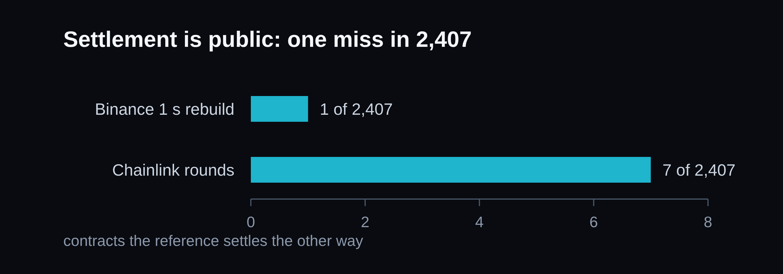
We rebuilt the rule from a public one-second Bitcoin series. It matched Polymarket's own settlements on 2,406 of the 2,407 contracts. Chainlink rounds, an independent reference, matched 2,400 of the same 2,407.
About 39% of these contracts are near-ties: price ends within 25 dollars of where it started, roughly one minute's normal move. In a near-tie the result comes down to a rounding difference, so a faster or cleaner feed is exactly what would win it.
We checked that door too. The public series still gets 2,406 of the 2,407 contracts right, near-ties included, and Chainlink gets 2,400. There is no contract left for a private feed to win.
The wallet's advantage is real. It wins about three times as often as its entry price implies, and that is not something a better feed would explain.
Test two: The math
The second test was better mathematics. A contract at one cent is a forecast: the market says that side is worth one percent. We built our own. Take the exact strike, write down the exact variance of the remaining 60-second average, estimate volatility from the recent past, fit one scale. Out comes a probability for each side at each moment.

K is the strike, the 60-second average at the window's open. St is the current reference price, σ̂ trailing realised volatility, R the seconds left in the window, L the 60-second averaging length, c one fitted scale, and Φ the standard normal distribution.
The denominator is not an assumption. The variance of the average over the last L seconds, given the price now, is exactly σ̂2(R − 2L/3) for R ≥ L. With no averaging window the bracket collapses to R, which is the ordinary random-walk answer.
Scored against a sampled last trade, the model won. Log loss 0.2299 against 0.2507. Log loss scores a forecast by how much probability it gave to the outcome that happened, and it punishes confident mistakes hardest; lower is better. The Brier score, the average squared error of those probabilities, improved by 0.0080, lower being better.
Then we changed the benchmark and the edge disappeared. A last trade is not a price. It is one print from an unknown moment, sometimes minutes old. The thing a trader can pay is the book mid, the midpoint between the best bid and the best ask. Scored against the mid, the model added nothing. The mid is already calibrated: when it says six percent, the event happens about six percent of the time.
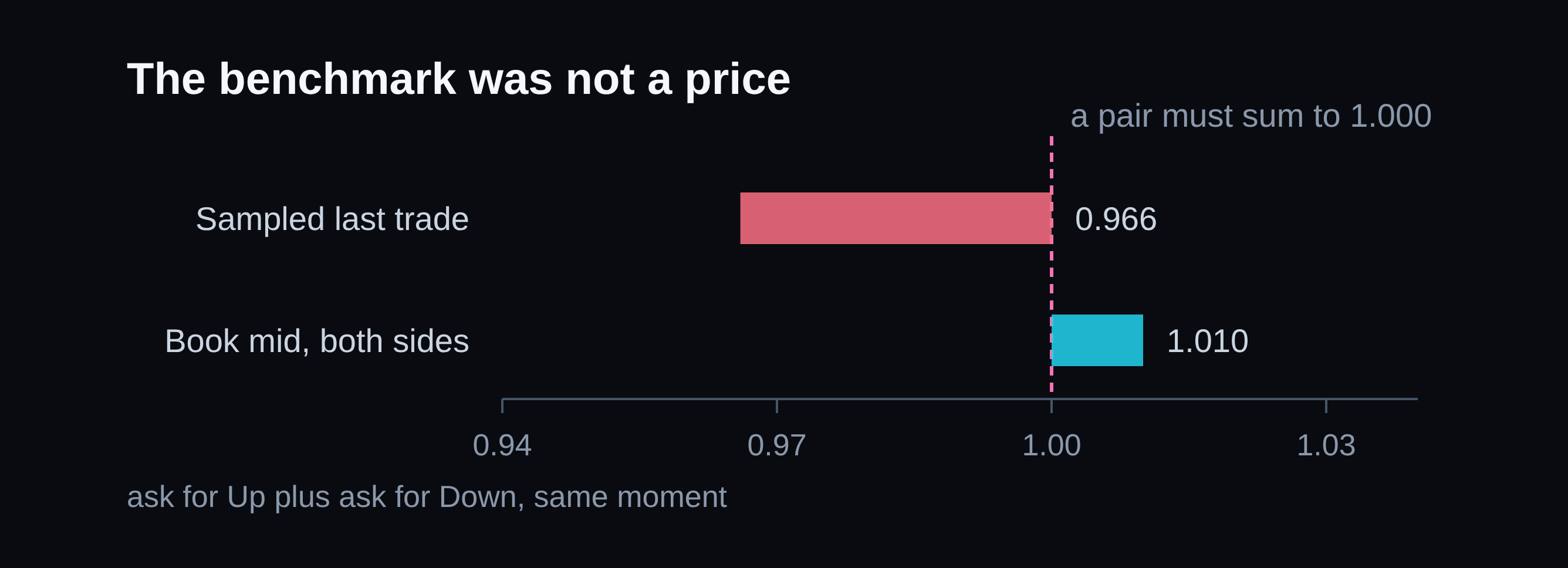
The model did not beat the market. It beat a bad copy of the market.
Test three: Our own method
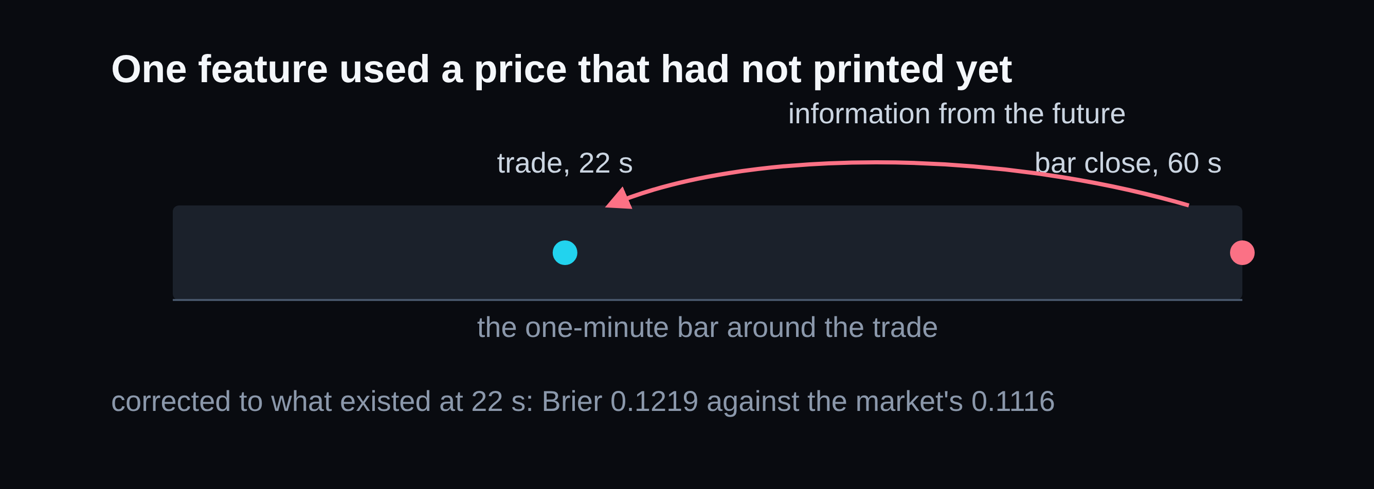
The third test was of our own method. A feature model beat the market out of sample, and it looked like the answer to the whole series. Then we read the feature list. One input was the closing price of the one-minute bar containing the trade. A trade partway into a window sits inside a minute that has not closed, so that price does not exist when the decision is made. The model was not predicting the future. It was remembering it.
Corrected to use only what was knowable at the trade, it scores a Brier of 0.1219 against the market's 0.1116 and loses $371.86 across 235 trades. That result changed how we tested everything after it, which is what makes it the useful one.

pt is price now, path the price path inside the window, σ̂ volatility, μ momentum, range high minus low, V volume, and τ time remaining. The target is the same as Test 2: the probability that the contract settles Up.
The defect is one coordinate. The model read close(⌊t⌋1m), the closing price of the minute containing the trade, which is not printed until that minute ends.
Five learners targeted the same thing: the probability that the contract settles Up. Boosted trees on seven inputs came first, then random forests, a small neural network, a polynomial, and a Bayesian logistic model that picked its own features and kept only the price. None of them beat the book mid.
The distributions answer a narrower question. The Φ in the formula above is a choice: it turns a standardized distance into a probability. We replaced it with a scaled normal, a skew-normal, a Student-t, and the raw empirical distribution of the same moves, holding the strike and the volatility estimate fixed. The plain normal scored best of the five, at a Brier of 0.1545 against the market's 0.1116. The other four were worse.
Test four: Speed
The fourth test was speed. If Bitcoin moves and the quote has not caught up, a fast buyer takes a contract at a price that is already wrong. That trade needs a gap between prints long enough to act in.
We measured the gaps. Half are zero seconds, 99 in 100 are three seconds or less, and 99.8 in 100 are ten seconds or less. Fewer than three gaps in ten thousand last longer than thirty seconds.
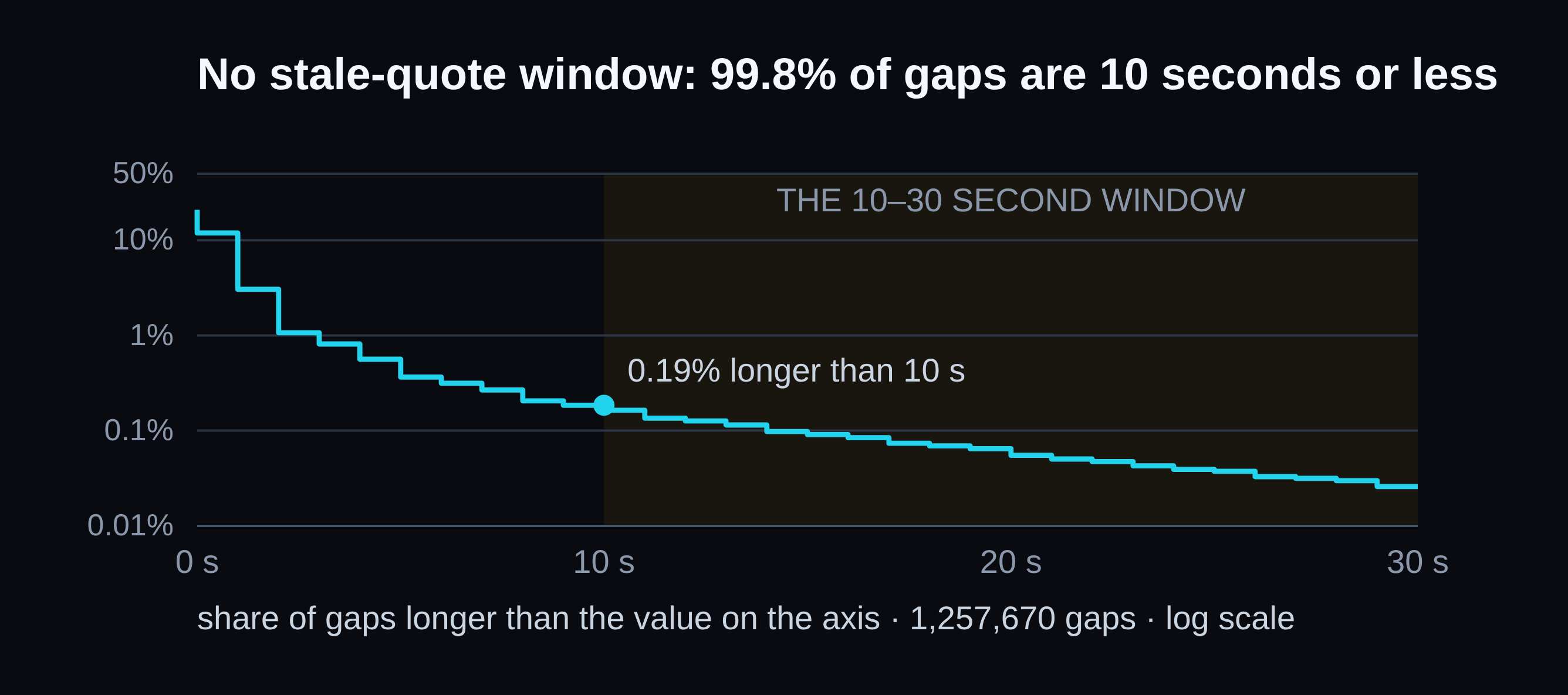
We tested the fastest version anyway. A model reading spot one second behind the market scores a Brier of 0.1152 against the market's 0.1116. One second late is already too late to know something the price does not.
Speed is not the answer either.
Test five: The crowd
The wallet may be reading something in data everyone else sees. So we built the sharpest test available: not whether it beats the price, which Part 1 settled, but whether its cheap entries differ from anyone else's at the same price and moment.
The wallet won 4 of 103. The matched controls won 3 of 142.
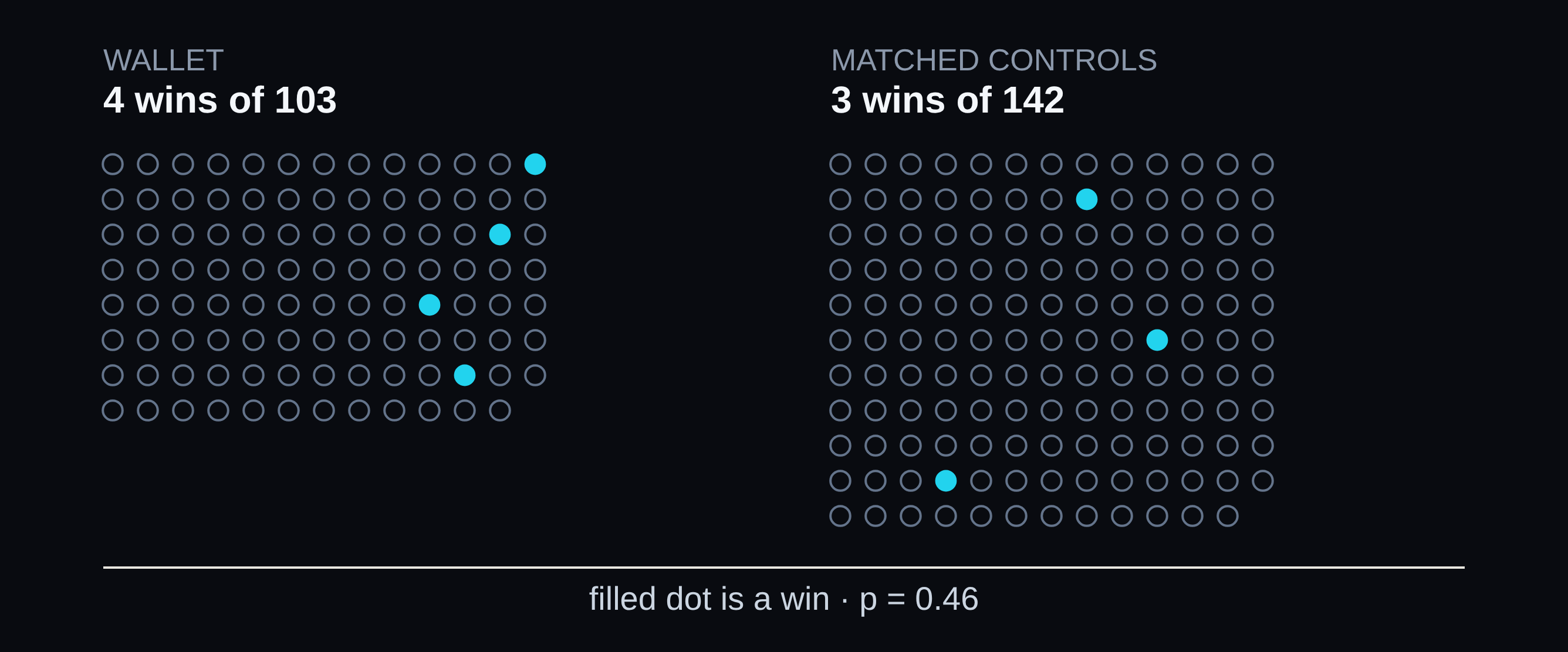
A p-value answers one narrow question: if there were no difference between the groups, how often would a gap this wide appear anyway? Here, 0.46. Nearly half the time. At four wins, a sample this size cannot separate them.
The crowd data went the wrong way too. We expected a wallet absorbing a seller, or joining a crowd that knew something. His entries are quieter than the controls: fewer prints, fewer wallets, no selling ahead of them.
Part 1 used an interval without naming it. That was a Wilson interval, which stays sane when wins are rare, unlike the textbook version that assumes a comfortable count of wins. At four wins, the honest statement is not that the wallet is twice as good. It is that we cannot tell.
The last door closed the same way. Polymarket settles the way we settle. The midpoint of the book is already right. Our first model was reading the future, and we caught it before it cost us the series. There is no speed race to run. And at the same price and moment, the wallet's entries are indistinguishable from everyone else's. Every door a trader normally walks through is closed, and the wallet is still on the other side of all of them.
If his entries look like everyone else's entries, the difference is not in the ticket.
Same instrument, same price, different moment. That is a harder thing to test, because the state is not in the ticket. It is where we should have looked first. Part 3 starts with a name that had been sitting in the first line of every data file since April.
Part 2 of 3. The windows are stated explicitly throughout. The $29,128 headline from Part 1 covers 4,707 positions from 17 July to 28 October. The band table covers 4,332 contracts from 23 July to 29 October. The settlement rows here cover the 30-day corpus of 2,407 contracts, and the gap measurement covers 934 contracts and 1.26 million print gaps from 30 October to 3 November. The windows differ on purpose, and every figure is reported as measured in the window it belongs to.