AWS Trading Part 2 - The Strategy

The code and diagrams for the strategy can be found on github. AWS Trading Part 2 Youtube video is here.
Introduction
In part 1 youtube video link we covered the data pipeline portion of the AWS trading bot architecture. I demonstrated how to set up your AWS environment, including creating a simple dynamoDB database to hold our price and strategy data. Then we walked through the data pipeline code in detail including how to grab the data and populate our db with it. In this post we’ll cover the strategy that we will be implementing.
Quick aside, you can choose a different DB, or data api. Perhaps you would prefer a relational database, and you have a subscription to a data provider like DTN Iqfeed or Databento. Those components can be changed at will because in this demo project I’ve attempted to make the code and system relatively modular so you can adapt it to your needs.
The Strategy
At the end of part 1 I needed to choose a strategy to implement. I wanted it to be something a little more interesting than a moving average crossover (which is basically the ‘hello world’ of algo trading). After brainstorming I decided on a market neutral long-only etf strategy.
Since it’s long only and we need it to be market neutral we take synthetic short positions by purchasing inverse ETFs. Overall the strategy is basically pairs trading strategy. Each pair is equally weighted. Within the pair we allocate market neutral weights accounting for the leverage in the inverse ETF. For example, in a 3x leverage inverse ETF, we allocate 3x the amount of cash to the unlevered ETF.
For example a $100 portfolio would invest $75 in XLF and $25 in FAZ.
The next obvious question is how does it make money? We’ll take a look at it in theory in the next section.
Exploratory Analysis
We have to consider market direction and volatility in understanding the sources of profit. Volatility is especially important because of the leveraged inverse leg. In theory we would expect the strategy to perform well in moderate to strongly trending markets. This strategy will get cooked in high volatility range bound markets. This is because of something called volatility decay, beta slippage or some other terms. Basically it’s the idea that for a sequence of returns there will be a gap between the underlying’s theoretical leveraged return and the return from the inverse ETF. This results from the fact that the inverse ETF has to rebalance daily to maintain the proper leverage by literally buying high and selling low. To explore this concept in more detail check out my blog post here.
In theory we expect the strategy to perform in rough accordance to this matrix based on market direction and volatility. A quick note, high vol in bullish or bearish trends should perform well because the price expansions are expected to cover the losses in the other leg.
This chart codifies the assumed outcomes using the pair XLF and FAZ. In bullish markets we expect the unlevered leg to outperform the losses in the levered leg and vice versa during the bearish trends. Moderate and low volatility regimes in a bearish market are dependent on the return sequence with a slight negative expectation because it’s expected that the gains from the inverse leg are less likely to outgain the losses in the unlevered leg. Sideways markets are likely to perform the worst because the inverse leg is losing value due to decay/slippage and the unlevered leg is not offsetting the damage.

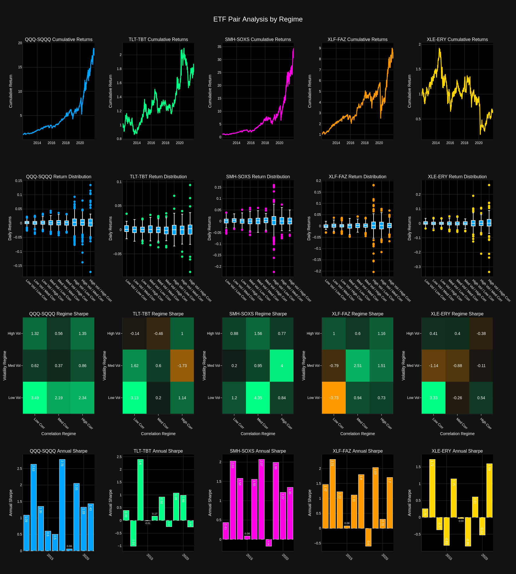
ETF PAIR ANALYSIS (DAILY RETURNS)
In the above chart (click the chart to enlarge) we further subdivide volatility and intra-pair correlation into regimes and look at the return volatility as well as the sharpe ratios. Quick observations, you would expect high vol, low correlation to have the widest range of returns but the QQQ-SQQQ, TLT-TBT, and XLY-ERY pairs don’t follow that convention. Interesting. XLE-ERY gets cooked in everyone medium volatility regime. XLF-FAZ struggled in mid to low vol environments with low correlation.

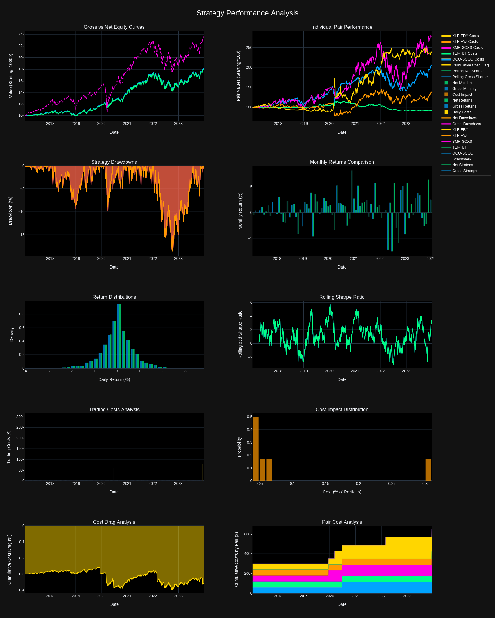
VISUAL RESULTS FROM ALL PAIRS BACKTEST 2017-2024. SIMULATED RESULTS. PAST PERFORMANCE IS NOT INDICATIVE OF FUTURE PERFORMANCE.
Strategy sharpe was about 0.8 over the period. I was somewhat surprised at the correlation between the strategy and SPY which was between 0.6-0.7.
Room For Improvement
- Portfolio weighting scheme is basic equal weight but may improve results by incorporating volatility and momentum.
- Vol regime filters could improve performance by lowering exposure during historically poor performance periods.
- Strategy is sensitive to rebalance frequency. The more frequent the rebalance the worse the performance.
Join the Conversation
Your feedback shapes this content! Whether you're stuck on a particular implementation detail or have ideas for future topics, I want to hear from you. Drop your thoughts in the comments below, join our Discord community, or reach out via email.
Stay tuned for Part 3, where we'll dive deeper into AWS deployment!
Want to learn more about automating your trading strategies? Check out my previous post on How I Automated My Trading Strategy Using AWS Cloud for Free, where I break down the initial system architecture and design decisions.
Enjoyed this post?
Subscribe for more research and trading insights.
By clicking "Subscribe," you agree to our Terms of Use and acknowledge our Privacy Policy. You can unsubscribe at any time.
No spam. Unsubscribe anytime.